---
title: "Tiered Persona Prompting for Communication Apprehension: A Digital-Twin Evaluation Against Classical Machine-Learning Baselines"
subtitle: "LLM persona agents and tabular baselines on PRCA ground truth across demographic, employment, geographic, and transportation tiers"
author:
- name: Jack J. Burleson
url: https://github.com/Exios66
affiliations:
- University of Wisconsin–Madison
corresponding: true
date: last-modified
abstract: |
Large language models (LLMs) are increasingly asked to stand in for human respondents
in survey and measurement research. This manuscript evaluates **tiered persona prompting
as a digital-twin method against classical machine-learning baselines** for recovering
self-reported communication apprehension (CA). Using McCroskey’s Personal Report of
Communication Apprehension (PRCA-24) *group* and *interpersonal* (IP) subscales (range 6–30),
we join Prolific demographics to Qualtrics
responses, build cumulative persona prompts (demographics → employment → geography →
transportation), and score LLM predictions against ground-truth PRCA alongside a
cross-validated tabular suite (Ridge, Elastic Net, k-NN, Random Forest [RF],
XGBoost, MLP).
Three primary research questions (RQ1–RQ3) examine whether employment status (RQ1),
transportation-use cues (RQ2), and full cumulative context including free-response
voice (RQ3) improve absolute CA prediction error — under either family — and how
prediction error distributes across demographic and contextual groups. Five secondary research questions (S1–S5) reverse the
predictive direction on the same matched sample, asking how CA, place, and mobility
self-reports relate to regular public-transit use (survey item Q26, weekly-or-more)
under classical
Random Forests rather than LLM inference. A further secondary *focus* pair (TF1–TF2)
asks whether models can estimate regular ridership and transit intensity from demographics,
context, and CA scores when transit / ride-share / car answers are held out of the prompt.
All displayed statistics use the full Prolific↔Qualtrics matched analytic cohort
(*N* = 241; 101 regular / 140 non-regular weekly+ transit riders).
Full-cohort GPU (vLLM, a high-throughput LLM serving engine) baselines on the original
prompt-`v1` five-tier ladder show that
none of four open-weight instruct/distill models is a high-fidelity digital twin
(exact match ≈6–9%). Among non-collapsed runs, **DeepSeek-R1-Distill-Llama-8B** achieves
the best pooled group-CA mean absolute error (MAE; 5.22) and the most tier-stable
profile; Llama-3.2-3B-Instruct
leads interpersonal (IP) MAE (5.35) and group band accuracy (52.7%); Llama-3.1-8B-Instruct
recovers interpersonal bands above chance early but collapses when transit cues are added
(IP MAE 4.67 → 8.17); Llama-3.3-70B-Instruct exhibits mode collapse (≈93% constant prior).
Every live model remains above the classical suite floor (best transit group MAE = 4.49
Ridge). Signal-first packaging (v2) with enhanced decoding and 8-tier ablation prompts (v3)
were GPU-evaluated from the archived `exports/` packages: DeepSeek improves under v2
(group MAE **5.02**; IP **5.26**; tier-stable), whereas v2 does **not** fix — and at the base
tier worsens — Llama-3.1's interpersonal error (demos IP 4.67 → **8.45**; transit 8.17 →
8.23). Greedy `v3` ablations show the Llama-3.1 collapse is **combination-specific**:
isolating ride-share (Q28), transit use (Q26), or open-text voice leaves IP MAE at
4.85–5.92, while the bundled mobility dump still collapses it (**7.77**); `v3_rideshare`
group MAE (5.86) also beats the kitchen-sink transit tier (**6.07**), matching the tabular
`Q28`-dominance result. On shared MAE/band metrics against the classical suite, the best
live agent (DeepSeek v2) trails on every tier, does not improve with richer tiers the way
Random Forest does, shows near-chance low-vs-high band discrimination (transit area
under the curve [**AUC**] **0.53** group / **0.49** interpersonal vs. RF **0.72** / **0.74**), and never
emits the high-CA band for
Group CA; surrogate
SHAP (SHapley Additive exPlanations)
on its outputs shows the agent over-weights geolocation and age relative to the
Q28/employment mix that predicts true CA. On the
same cohort, traditional Random Forests show that ride-share days (Q28) predict regular
transit at cross-validated receiver-operating-characteristic **area under the curve** (**CV ROC-AUC**) = **0.762**,
whereas transit-day intensity (Q27) yields AUC = **0.589**;
geography (**0.551**) and CA scores (**0.590**) remain near chance. Extended follow-ups show Q28
retains lift after car access, demographics (especially age) modestly predict ridership,
and CA adds little once Q28 is known. A kitchen-sink mobility+demo forest reaches AUC =
0.824 but remains Q28-dominated. Holding mobility self-reports out (TF1), a profile of
demos + employment + geo still reaches regular-transit AUC = **0.662** (**0.672** with CA);
fine-grained intensity (TF2) remains weak. Together, the primary and secondary results
clarify which mobility cues belong in persona tiers and which reverse predictors of
transit habits carry the strongest tabular signal in this sample.
keywords:
- communication apprehension
- large language models
- digital twin
- persona prompting
- PRCA-24
- algorithmic bias
- machine learning baselines
- public transit
- ride-share
- random forests
- Prolific
- Qualtrics
- PSYCH 755
nocite: |
@*
toc: true
toc-depth: 3
bibliography: references.bib
---
```{python}
#| label: setup
#| include: false
from __future__ import annotations
import json
import sys
from pathlib import Path
import matplotlib.pyplot as plt
import numpy as np
import pandas as pd
ROOT = Path.cwd()
SRC = ROOT / "src"
if str(SRC) not in sys.path:
sys.path.insert(0, str(SRC))
from ca_personas.apa_plotting import (
apa_axes,
apply_apa_style,
grouped_bars,
horizontal_bars,
scatter_identity,
)
from ca_personas.paths import (
cohort_source_label,
full_cohort_paths,
sibling_data_available,
)
from ca_personas.personas import CORE_TIERS, build_persona_prompt
from ca_personas.pipeline import run_pipeline
apply_apa_style()
RENDER_OUT = ROOT / "outputs" / "quarto_render"
COMMITTED_FULL = ROOT / "artifacts" / "posit_full_cohort"
SECONDARY_PATH = COMMITTED_FULL / "secondary_results.json"
if sibling_data_available():
PROLIFIC, QUALTRICS = full_cohort_paths()
DATA_SOURCE = cohort_source_label()
artifacts = run_pipeline(
prolific_path=PROLIFIC,
qualtrics_path=QUALTRICS,
tiers=list(CORE_TIERS),
provider="mock",
output_dir=RENDER_OUT,
join_how="inner",
)
participants = pd.read_csv(artifacts["participants"])
evaluation = pd.read_csv(artifacts["evaluation"])
summary = pd.read_csv(artifacts["summary"])
else:
required = [
COMMITTED_FULL / "participants.csv",
COMMITTED_FULL / "evaluation.csv",
COMMITTED_FULL / "summary.csv",
COMMITTED_FULL / "source.json",
SECONDARY_PATH,
]
missing = [p for p in required if not p.is_file()]
if missing:
raise FileNotFoundError(
"Full-cohort File A/B/C not staged and committed Posit artifacts "
f"are missing: {missing}"
)
meta = json.loads((COMMITTED_FULL / "source.json").read_text(encoding="utf-8"))
if meta.get("data_source") == "excerpts" or int(meta.get("n_analytic", 0)) < 100:
raise RuntimeError(f"Refusing excerpt-scale Posit artifacts: {meta}")
DATA_SOURCE = meta.get("data_source", "artifacts/posit_full_cohort")
participants = pd.read_csv(COMMITTED_FULL / "participants.csv")
evaluation = pd.read_csv(COMMITTED_FULL / "evaluation.csv")
summary = pd.read_csv(COMMITTED_FULL / "summary.csv")
artifacts = {
"participants": COMMITTED_FULL / "participants.csv",
"evaluation": COMMITTED_FULL / "evaluation.csv",
"summary": COMMITTED_FULL / "summary.csv",
"source": COMMITTED_FULL / "source.json",
"secondary": SECONDARY_PATH,
}
if len(participants) < 100:
raise RuntimeError(
f"Analytic N={len(participants)} looks like an excerpt demo; "
"Posit pages must use the full matched cohort."
)
if not SECONDARY_PATH.is_file():
raise FileNotFoundError(
f"Missing {SECONDARY_PATH}. Run scripts that sync full-cohort secondary results."
)
secondary = json.loads(SECONDARY_PATH.read_text(encoding="utf-8"))
_secondary_n = int(secondary.get("n_analytic", 0))
if _secondary_n and _secondary_n != len(participants):
raise RuntimeError(
f"secondary_results.json n_analytic={_secondary_n} does not match "
f"participants N={len(participants)}; re-sync artifacts before render."
)
N = int(len(participants))
```
::: {.github-access}
<a class="github-btn" href="https://github.com/Exios66/psych755-jjb" target="_blank" rel="noopener" aria-label="Open the psych755-jjb GitHub repository">
<i class="bi bi-github" aria-hidden="true"></i>
<span>Repository</span>
</a>
<a class="github-btn" href="https://github.com/Exios66" target="_blank" rel="noopener" aria-label="Open Jack Burleson GitHub profile Exios66">
<i class="bi bi-github" aria-hidden="true"></i>
<span>Exios66</span>
</a>
:::
# Introduction
Communication apprehension (CA) is a well-studied individual difference describing fear or anxiety associated with real or anticipated communication [@mccroskey1970; @mccroskey1984]. McCroskey first introduced the Personal Report of Communication Apprehension (PRCA-24) in the fourth edition of *An Introduction to Rhetorical Communication* [@mccroskey1982], and the measure remains the standard self-report tool for the construct, with the current scoring guide maintained by the author [@mccroskeyprca24]. Early self-report batteries for social-communicative anxiety were compared and validated in the late 1970s [@daly1978], and the PRCA-24's content validity across communication contexts was subsequently established [@mccroskey1984]. The PRCA-24 yields context-specific subscale scores—including *group discussion* and *interpersonal* conversation—each ranging from 6 (very low apprehension) to 30 (very high) [@mccroskey1982; @beatty1988].
Separately, large language models are increasingly used as **survey respondents** and **silicon samples**: prompts that condition on demographic or biographical attributes and emit attitude- or item-like answers [@argyle2023; @park2024; @chuang2026aiterrarium]. A converging program statement argues that LLM social simulations are a promising—and by now widely deployed—research method [@anthis2025; @grossmann2023], with applications spanning augmented-democracy deliberation [@gudino2024] and hybrid "AI-augmented" survey pipelines that pair generative models with traditional self-report instruments [@kim2023aisurveys; @kaiser2025]. Related work on generative agents and digital-twin simulation explores whether models can stand in for populations or individuals in social-science workflows [@park2023; @park2024; @binz2024], and behavioral economists have pushed the same agenda in experimental economics, treating instruction-tuned models as implicit computational models of humans ("*homo silicus*") whose behavior can be probed in simulated scenarios [@horton2023]. Across these pipelines, a consistent finding is that **demographics alone are insufficient**: aligning role-playing agents on human *belief networks*—structured beliefs about the world and others—improves predictive fidelity over demographic-only personas [@chuang2024belief], and personalized survey-data modeling is explicitly framed as the payoff of such richer profiles [@kaiser2025]. There is also positive capability evidence: zero-shot models can already outperform human experts and crowd workers on social-science annotation tasks [@tornberg2023]. At the same time, a parallel literature documents **perils**: synthetic replacements for human survey samples inherit and distort population distributions rather than preserving them [@bisbee2024], simulated opinions diverge from measured public opinion and carry systematic biases [@qu2024opinion; @lee2025ideology], persona prompts surface social stereotypes and opinion distributions that do not faithfully track the populations they purport to represent [@cheng2023; @santurkar2023; @hu2024; @salewski2023], and outputs are sensitive to prompt packaging and position [@sclar2024]. The same persona-impersonation mechanisms that recover human-like developmental or expertise effects can also reveal systematic group biases [@salewski2023], and formatting-level prompt variation alone shifts downstream answers in measurable ways [@sclar2024]. That raises a concrete measurement question for psychological research tooling:
> When predicting an individual’s CA from demographic attributes alone, does an LLM’s prediction error vary systematically with demographic or contextual group membership — and does the model recover the same covariate signal that classical baselines extract?
Methodologically, this manuscript sits between two traditions. The *data-modeling culture* [@breiman2001cultures] treats the task as estimating a stochastic relationship between covariates and an outcome and focuses on parameter inference; the *algorithmic-modeling culture* [@breiman2001cultures; @breiman2001] treats it as a predictive function-learning problem and focuses on out-of-sample error. We deliberately adopt both: classical tabular learners (Ridge, Elastic Net, k-nearest neighbors, Random Forest, and gradient-boosted trees) supply the algorithmic floor under cross-validation, while the reverse-predictor secondary analyses add inferential contrasts (Welch *t* tests, effect sizes, bootstrap CIs) of the data-modeling kind. The LLM persona agents are evaluated as a third, predictive family against the same ground truth, so digital-twin error can be benchmarked against a classical algorithmic baseline rather than judged in a vacuum [@argyle2023; @breiman2001cultures; @park2023]—a design that answers the call to validate synthetic survey substitutes against observed respondent data rather than against the models themselves [@bisbee2024; @qu2024opinion]. In the terminology of recent cognitive-model work, we are asking not whether LLMs can be *turned into* cognitive models of the PRCA-24 [@binz2024; @argyle2023] but how close a persona-conditioned inference family comes to a classical learner on the same held-out psychometric target.
## Research Questions
The primary design compares **information tiers** rather than a single prompt: each participant is personified five ways (`demos` → `employment` → `geo` → `transit` → `full`) while ground-truth PRCA stays fixed, directly testing the "beyond demographics" result that accumulating non-demographic context—beliefs, circumstances, and behavior—improves persona fidelity [@chuang2024belief; @kaiser2025]. The present study addressed three primary research questions — whether adding employment status (RQ1), transportation-use cues (RQ2), or full cumulative context including free-response voice (RQ3) shrinks prediction error relative to classical ML, and whether residual error still clusters by group membership; five secondary research questions concerning classical predictors of regular public-transit use; and a secondary *focus* pair that holds transit self-reports out of the persona/profile and asks models to estimate ridership instead [@cheng2023; @santurkar2023]. Because persona prompting is known to be packaging-sensitive [@hu2024; @argyle2023; @sclar2024], the project also evaluates signal-first redesigns (`v2`/`v3`) against the published v1 baselines.
::: {.research-focus-block}
### Primary Research Questions
*Outcome.* Continuous PRCA-24 group and interpersonal communication apprehension scores (range 6–30).
*Design.* Cumulative persona prompts (`demos` → `employment` → `geo` → `transit` → `full`) evaluated with mean absolute error (MAE), signed error, and band accuracy against Qualtrics ground truth; each tier after `demos` maps to a primary RQ (RQ1 = `employment`, RQ2 = `transit`, RQ3 = `full`).
**Research Question 1 (RQ1):** Does adding employment status to a basic-demographics persona improve an LLM's predictive accuracy for self-reported communication apprehension scores, and does residual prediction error cluster systematically by employment group membership?
**Research Question 2 (RQ2):** Does adding transportation-use information to the geo-context persona improve prediction of communication apprehension relative to earlier tiers, and does the model use mobility cues in a psychologically sensible way rather than as stereotype proxies?
**Research Question 3 (RQ3):** Does adding full cumulative context — including free-response attitudes (voice text) beyond the transit tier — improve prediction of communication apprehension, or are the combined cues redundant?
:::
::: {.research-focus-block}
### Secondary Research Questions
*Outcome.* Binary regular public-transit use from Qualtrics `Q26` (`4-8 days a month` or `8 or more days a month`).
*Design.* Classical random forests (RF) with stratified 5-fold cross-validation
(`random_state=42`) on the Prolific↔Qualtrics matched analytic sample (*N* = 241)—not
LLM inference [@breiman2001; @pedregosa2011; @prolific].
**Research Question 1 (S1):** Do regular public-transit riders differ from non-regular riders in group and interpersonal communication apprehension?
**Research Question 2 (S2):** Does survey geolocation (latitude and longitude) predict regular public-transit use?
**Research Question 3 (S3):** Do group and interpersonal communication apprehension scores predict regular public-transit use?
**Research Question 4 (S4):** Do transit-day intensity (Q27) and ride-share days (Q28) predict regular public-transit use?
**Research Question 5 (S5):** Do Wave-2 covariates—demographics, country versus coordinates, ride-share days conditional on car access, joint CA and mobility models, and residual CA after ride-share—improve prediction of regular public-transit use beyond the Wave-1 mobility predictors?
:::
::: {.research-focus-block}
### Secondary Focus — Transit Prediction with Mobility Held Out
*Outcome.* Binary regular public-transit use (`Q26` weekly+) and ordinal transit intensity (`Q26` day-frequency; `Q27` rides/day).
*Design.* Profile features and persona prompts that include demographics, employment, geography, and (for intensity / CA arms) PRCA scores — with **Q26–Q29, Q20, Q21, and Q19 held out**. Classical Random Forests establish the tabular ceiling; parallel transit-focus LLM prompts (`tf_demos` → `tf_geo_ca`) are generated for future GPU twins ([write-up](docs/secondary_rq_transit_focus.md); [memo](memos/transit_focus_regular_and_intensity.qmd)).
**Focus Question 1 (TF1):** Given contextual information and a user profile with transit questions held out of the prompt, can models estimate whether the user is a regular public-transit rider? (Seeded RF area under the curve [AUC] = **0.662** profile-only; **0.672** with CA; *n* = 224.)
**Focus Question 2 (TF2):** Given demographics, context, and CA scores — still holding transit self-reports out — can models estimate the user’s public-transit use intensity (Q26 / Q27)? (Seeded RF Q26 balanced accuracy = **0.283**, ordinal MAE = **1.22**; Q27 remains majority-class dominated.)
:::
Supporting methods pages: [cohort EDA](docs/cohort_eda.md), [ML baselines](docs/ml_baselines.md), [ML vs LLM metrics](docs/ml_vs_llm.md), and [feature importance](docs/factor_feature_importance.md). Secondary write-ups: [S1](docs/secondary_rq_transit_ca.md), [S2](docs/secondary_rq_geo_predicts_transit.md), [S3](docs/secondary_rq_ca_predicts_transit.md), [S4](docs/secondary_rq_q27_q28_predict_transit.md), [S5](docs/secondary_rq_followup_experiments.md), [TF1/TF2](docs/secondary_rq_transit_focus.md). Code and site source: [github.com/Exios66/psych755-jjb](https://github.com/Exios66/psych755-jjb) [@psych755repo]; author profile: [github.com/Exios66](https://github.com/Exios66) [@github].
# Methods
## Data sources
Participants were recruited via Prolific [@prolific] in two waves (File A + File B; stacked) and completed a Qualtrics [@qualtrics] instrument (File C). Private full-cohort exports are not committed to git. **All statistics on this site use the full matched analytic cohort**: 252 Prolific∩Qualtrics matches → *N* = 241 with complete scorable PRCA. The join key is Prolific `Participant id` ↔ Qualtrics `Q0`. Cleaning retains inner-join respondents with complete PRCA group and interpersonal items so every information tier shares the same ground-truth targets.
```{python}
#| label: tbl-sample
#| tbl-cap: "Analytic Sample Composition for the Full Matched Cohort"
#| tbl-colwidths: [40, 60]
def _label_counts(series: pd.Series) -> pd.Series:
    """Value counts with missing coded as Missing (avoid displaying 'nan')."""
    labeled = series.fillna("Missing").astype(str).replace({"nan": "Missing", "<NA>": "Missing"})
    return labeled.value_counts(dropna=False)


sex_counts = _label_counts(participants["Sex"])
emp_counts = _label_counts(participants["Employment status"])
stu_counts = _label_counts(participants["Student status"])
cty_counts = _label_counts(participants["Country of residence"]).head(5)
pd.DataFrame(
    [
        {"Metric": "Analytic N (complete PRCA)", "Value": f"{N}"},
        {
            "Metric": "Group CA *M* (*SD*)",
            "Value": f"{participants['gt_group_ca'].mean():.2f} ({participants['gt_group_ca'].std():.2f})",
        },
        {
            "Metric": "Interpersonal CA *M* (*SD*)",
            "Value": f"{participants['gt_interpersonal_ca'].mean():.2f} ({participants['gt_interpersonal_ca'].std():.2f})",
        },
        {
            "Metric": "Sex",
            "Value": "; ".join(f"{k} = {v}" for k, v in sex_counts.items()),
        },
        {
            "Metric": "Student status (base demos)",
            "Value": "; ".join(f"{k} = {v}" for k, v in stu_counts.items()),
        },
        {
            "Metric": "Employment status",
            "Value": "; ".join(f"{k} = {v}" for k, v in emp_counts.items()),
        },
        {
            "Metric": "Top countries of residence",
            "Value": "; ".join(f"{k} = {v}" for k, v in cty_counts.items()),
        },
        {
            "Metric": "Regular transit prevalence (Q26 weekly+)",
            "Value": f"{secondary['n_regular']}/{N} = {secondary['prevalence']:.3f}",
        },
    ]
)
```
::: {.callout-note}
## Full cohort only
Every table and figure uses the File A/B/C matched analytic sample (*N* = 241). Posit Connect Cloud loads committed artifacts under `artifacts/posit_full_cohort/` when private exports are absent. Excerpt fixtures are reserved for unit tests and are never displayed here.
:::
## Ground-truth PRCA scoring
Group items (`Q1`–`Q6`) and interpersonal items (`Q13`–`Q18`) use five-point Likert labels mapped to 1–5. Comfort-oriented items are reverse-coded as $6 - x$. Each subscale is the sum of six items (range 6–30). Classroom bands follow **low** (≤13), **moderate** (14–19), and **high** (≥20).
## Data cleaning and preparation
Before analysis, the stacked Prolific waves (File A + File B) were joined to the Qualtrics responses (File C) on the Prolific `Participant id` ↔ Qualtrics `Q0` key using an inner join. We retained only respondents with complete group (`Q1`–`Q6`) and interpersonal (`Q13`–`Q18`) PRCA items so that every information tier shares the same ground-truth targets, yielding *N* = 241. Demographic fields (Age, Sex, Country of residence, Student status, Employment status) were carried from the Prolific profile; geolocation (latitude/longitude) and the mobility/transit items (`Q20`, `Q21`, `Q26`–`Q29`) came from the Qualtrics survey. Free-response items (`Q18_advice`, `Q19`) were kept as raw text for the `full` persona tier and were not used as tabular predictors. Cleaning produced the analytic sample described in @tbl-sample, with no imputation of PRCA items and no exclusion beyond missing PRCA responses on the inner-join match.
```{python}
#| label: tbl-clean
#| tbl-cap: "Data Cleaning and Analytic Sample Steps"
#| tbl-colwidths: [40, 60]
pd.DataFrame(
    [
        {"Step": "Recruit via Prolific", "Detail": "Two waves (File A + File B), stacked on Prolific demographics"},
        {"Step": "Survey via Qualtrics", "Detail": "File C: PRCA-24 items, mobility items (Q20/Q21/Q26–Q29), free-response voice"},
        {"Step": "Join", "Detail": "Inner join on Prolific `Participant id` ↔ Qualtrics `Q0`"},
        {"Step": "Raw matches", "Detail": "252 Prolific ∩ Qualtrics"},
        {"Step": "Complete PRCA", "Detail": "241 with complete group + interpersonal items (analytic N)"},
        {"Step": "Scoring", "Detail": "Likert 1–5; comfort items reverse-coded 6 − x; subscale sums 6–30"},
        {"Step": "Bands", "Detail": "**low** (≤13) · **moderate** (14–19) · **high** (≥20)"},
    ]
)
```
## Statistical methods
Analyses follow the two modeling cultures [@breiman2001cultures; @breiman2001]. **Primary RQ1–RQ3** are predictive, algorithmic-culture comparisons: we optimize **mean absolute error (MAE)** and band-level accuracy/macro-F1 on the PRCA group and interpersonal targets, with exact-match rate and band distance reported as secondary diagnostics. The classical tabular suite (Ridge, Elastic Net, k-nearest neighbors, Random Forest, HistGradientBoosting, XGBoost, MLP) supplies the **baselines**, evaluated under the same tiers/targets; the best classical floor is Ridge at `transit` (group MAE ≈ 4.49). **Secondary S1–S5 and TF1–TF2** are reverse-prediction analyses on regular public-transit use (binary `Q26` weekly+; prevalence 0.419). Classification uses stratified 5-fold cross-validated Random Forests (`random_state=42`) reporting **ROC-AUC**, average precision, balanced accuracy, and F1; chance = 0.500. Where inferential statistics are used (S1; wave-2 Welch contrasts), we report Welch's *t*, *df*, Cohen's *d*, and 95% bootstrap CIs (1,000 resamples) for mean differences, with $\alpha$ = .05 two-tailed.
**Hypotheses.** For each research question we test the null against the alternative below. Primary questions are evaluated against the classical ML floor rather than against chance; secondary classification questions are evaluated against the chance AUC of 0.500; S1 is a two-tailed mean difference test.
| RQ | Null hypothesis (H₀) | Alternative hypothesis (H₁) |
|---|---|---|
| RQ1 · employment | Adding employment status does not change MAE vs `demos` (ΔMAE = 0). | Employment reduces MAE (ΔMAE < 0) and/or changes residual patterns across employment groups. |
| RQ2 · transit | Adding the mobility bundle does not change MAE vs `geo` (ΔMAE = 0). | Transit cues reduce MAE (ΔMAE < 0) in a psychologically sensible way, not as stereotype proxies. |
| RQ3 · full | Adding free-response voice does not change MAE vs `transit` (ΔMAE = 0). | Voice text reduces MAE (ΔMAE < 0). |
| S1 · transit ↔ CA | Regular riders' group/interpersonal CA equals non-regular riders' (μ₁ = μ₂). | Regular riders differ in CA (μ₁ ≠ μ₂). |
| S2 · geo → transit | Lat/long RF ROC-AUC = 0.500. | Lat/long ROC-AUC > 0.500. |
| S3 · CA → transit | CA RF ROC-AUC = 0.500. | CA ROC-AUC > 0.500. |
| S4 · Q27/Q28 → transit | Q27/Q28 RF ROC-AUC = 0.500. | Ride-share days and/or intensity ROC-AUC > 0.500. |
| S5 · follow-ups | Wave-2 covariates add no lift over wave-1 predictors (ΔAUC = 0). | Covariates improve ROC-AUC (ΔAUC > 0). |
| TF1 · profile → transit | Profile-only RF ROC-AUC = 0.500. | Non-mobility profile ROC-AUC > 0.500. |
| TF2 · transit intensity | Intensity model performs at the majority-class baseline (ordinal MAE). | Intensity is recoverable beyond the majority baseline. |
: Null and alternative hypotheses for every research question. {#tbl-hypotheses}
Because the primary comparisons benchmark two predictive families on the same fixed ground truth, we report point estimates with cross-validation standard errors rather than *p* values for RQ1–RQ3; inferential *p* values are reported only where a stochastic contrast (Welch) is the appropriate model [@breiman2001cultures; @breiman2001].
```{python}
#| label: tbl-gt-summary
#| tbl-cap: "Descriptive Statistics for Ground-Truth PRCA Subscales (*N* = 241)"
gt = (
    participants[["gt_group_ca", "gt_interpersonal_ca"]]
    .rename(
        columns={
            "gt_group_ca": "Group CA",
            "gt_interpersonal_ca": "Interpersonal CA",
        }
    )
    .describe()
    .T[["count", "mean", "std", "min", "25%", "50%", "75%", "max"]]
    .round(2)
)
gt
```
```{python}
#| label: tbl-correlation
#| tbl-cap: "Base-Reference Spearman Correlations Among Continuous and Ordinal Measures"
#| tbl-colwidths: [30, 14, 14, 14, 14, 14, 14]
def _ord(series: pd.Series, mapping: dict) -> pd.Series:
    return series.map(mapping).astype(float)

q26ord = {"Never": 0, "0-1 days a month": 1, "2-4 days a month": 2, "4-8 days a month": 3, "8 or more days a month": 4}
q28ord = dict(q26ord)
q27ord = {"1-2 rides in a typical day": 1, "3-4 rides in a typical day": 2, "5-6 rides in a typical day": 3, "7 or more rides in a typical day": 4}

corr_vars = pd.DataFrame(
    {
        "Group CA": participants["gt_group_ca"],
        "IP CA": participants["gt_interpersonal_ca"],
        "Age": participants["Age"],
        "Q26 transit days": _ord(participants["Q26"], q26ord),
        "Q27 rides/day": _ord(participants["Q27"], q27ord),
        "Q28 ride-share days": _ord(participants["Q28"], q28ord),
    }
)
corr_mat = corr_vars.corr(method="spearman").round(2)
corr_mat.style.set_properties(**{"text-align": "center"}).format(precision=2)
```
*Note.* Spearman *ρ* on complete ordinal codings of the mobility items (`Q26` transit-use days, `Q27` rides on a typical day, `Q28` ride-share days). Regular transit (`Q26` weekly+) and ride-share days are positively related (*ρ* ≈ 0.6–0.7); the PRCA subscales are strongly inter-correlated (*ρ* ≈ 0.6) and largely orthogonal to demographics and mobility cues — consistent with CA operating as a distinct trait rather than a proxy for transit exposure.
```{python}
#| label: tbl-group-descriptives
#| tbl-cap: "Descriptive Statistics by Regular-Transit Group (*N* = 241)"
#| tbl-colwidths: [35, 20, 20, 25]
def _fmt(series: pd.Series, mask: pd.Series) -> str:
    sub = series[mask].dropna()
    return f"{sub.mean():.2f} ({sub.std():.2f})" if len(sub) else "—"

regular = _ord(participants["Q26"], {"Never": 0, "0-1 days a month": 0, "2-4 days a month": 0, "4-8 days a month": 1, "8 or more days a month": 1}).astype(bool)
pd.DataFrame(
    [
        {
            "Measure": "Group CA",
            "Regular (n = 101)": _fmt(participants["gt_group_ca"], regular),
            "Not regular (n = 140)": _fmt(participants["gt_group_ca"], ~regular),
            "Δ (reg − not)": f"{secondary['transit_ca']['group']['diff_regular_minus_not_regular']:.2f}",
        },
        {
            "Measure": "Interpersonal CA",
            "Regular (n = 101)": _fmt(participants["gt_interpersonal_ca"], regular),
            "Not regular (n = 140)": _fmt(participants["gt_interpersonal_ca"], ~regular),
            "Δ (reg − not)": f"{secondary['transit_ca']['interpersonal']['diff_regular_minus_not_regular']:.2f}",
        },
        {
            "Measure": "Age",
            "Regular (n = 101)": _fmt(participants["Age"], regular),
            "Not regular (n = 140)": _fmt(participants["Age"], ~regular),
            "Δ (reg − not)": "",
        },
        {
            "Measure": "Q28 ride-share days (ordinal 0–4)",
            "Regular (n = 101)": _fmt(_ord(participants["Q28"], q28ord), regular),
            "Not regular (n = 140)": _fmt(_ord(participants["Q28"], q28ord), ~regular),
            "Δ (reg − not)": "",
        },
    ]
)
```
## Persona tiers
Persona prompts follow the **AI Terrarium** digital-twin framing [@chuang2026aiterrarium]: the *user* message is a fluent second-person narrative (“You are a …”) plus a short CA self-report ask — not a bullet-list profile [@quarto]. Prompt **versions** are documented in [`docs/persona_prompt_versions.qmd`](docs/persona_prompt_versions.qmd): **v1** (original 5-tier ladder; all primary live baselines), **v2** (same five fields with signal-first packaging — GPU-evaluated on Llama-3.1/3.2/DeepSeek, `exports/v2/`), and **v3** (adds three ablations → eight tiers — greedy GPU runs on three models, `exports/v3/`; canonical ``v3_enhanced`` refresh pending). Full Prolific waves omit ethnicity / nationality / language; the `demos` tier uses Age, Sex, Country of residence, and Student status. Samples: [`prompts/examples/`](prompts/examples/).
| # | Tier | Role |
|:--:|---|---|
| 1 | `demos` | Base demographics |
| 2 | `employment` | + employment status (RQ1) |
| 3 | `geo` | + approximate survey lat/long (1 decimal) |
| 4 | `transit` | + full mobility bundle (RQ2) |
| 5 | `full` | + free-response attitudes (RQ3) |
| 6 | `v3_rideshare` | `geo` base + Q28 only (`v3` ablation) |
| 7 | `v3_public_transit` | `geo` base + Q26 only (`v3` ablation) |
| 8 | `v3_voice` | `geo` base + Q18.1/Q19 only (`v3` ablation) |
: Persona prompt tiers used across all live LLM baselines (v1/`v2`/`v3`). {#tbl-tiers}
The listings below show the **core ladder** (`CORE_TIERS`) for the **same** analytic participant so each step visibly accumulates context. Parallel `v3` ablations are illustrated in [`docs/persona_prompt_efficiency.md`](docs/persona_prompt_efficiency.md).
```{python}
#| label: persona-tier-progression
#| output: asis
from ca_personas.personas import CORE_TIERS, build_persona_prompt, voice_sentences

# Prefer a participant whose core user prompts strictly grow in length and
# whose `full` tier includes free-response voice — progressive stack only
# (`v3` ablations are parallel tips, not cumulative steps after geo).
tier_labels = {
    "demos": "1. demos — base demographics",
    "employment": "2. employment — demos + work status",
    "geo": "3. geo — employment + place coordinates",
    "transit": "4. transit — geo + mobility self-reports",
    "full": "5. full — transit + free-response attitudes",
}

example_row = None
example_prompts = None
for _, row in participants.iterrows():
    if not voice_sentences(row):
        continue
    built = {t: build_persona_prompt(row, t) for t in CORE_TIERS}
    lengths = [len(built[t].user_prompt) for t in CORE_TIERS]
    if all(lengths[i] < lengths[i + 1] for i in range(len(lengths) - 1)):
        if all(built[t].user_prompt.lstrip().startswith("You are") for t in CORE_TIERS):
            example_row = row
            example_prompts = built
            break

if example_row is None or example_prompts is None:
    example_row = participants.iloc[0]
    example_prompts = {t: build_persona_prompt(example_row, t) for t in CORE_TIERS}

pid_short = str(example_row["participant_id"])[:12] + "…"
print(
    f"*Same participant throughout (`{pid_short}`); core ladder user messages only — "
    "second-person persona narrative + CA ask (system prompt omitted).*\n"
)

for tier in CORE_TIERS:
    user = example_prompts[tier].user_prompt.strip()
    if not user.startswith("You are"):
        raise AssertionError(f"Expected Terrarium narrative for tier={tier}")
    stale_markers = ("Demographics:", "Adopt the following", "Fully personify")
    if any(marker in user for marker in stale_markers):
        raise AssertionError(f"Stale checklist-style prompt leaked for tier={tier}")
    print(f"### {tier_labels[tier]}\n")
    print("```text")
    print(user)
    print("```\n")
```
## Model calling and classical baselines
The Python package `ca_personas` supports Ollama, OpenRouter, and a deterministic **mock** provider used only for offline smoke tests and credential-free CI checks [@ollama; @openrouter]. Predicted JSON fields are validated to the legal 6–30 range, then joined to ground truth for signed and absolute errors. All displayed statistics on this site are computed from committed full-cohort vLLM exports, seeded tabular runs, and committed artifact tables so Cloud builds remain keyless — no mock predictions are reported.
A seven-model tabular suite (Ridge, Elastic Net, k-NN, Random Forest, HistGradientBoosting, XGBoost, MLP) on the same tiers and targets is reported in [`docs/ml_baselines.md`](docs/ml_baselines.md). On the full cohort, the **best** group-CA MAE reaches **4.49** at `transit` (Ridge; RF = 4.68); the best interpersonal MAE reaches **4.25** (Elastic Net; MLP = 4.31). Feature attributions and ML-vs-LLM comparisons are documented in [`docs/factor_feature_importance.md`](docs/factor_feature_importance.md), [`docs/ml_vs_llm.md`](docs/ml_vs_llm.md), and [`memos/feature_predictive_power_ml_llm.qmd`](memos/feature_predictive_power_ml_llm.qmd).
Full-cohort **live** LLM baselines use GPU **vLLM** exports on the original prompt-**`v1`** five-tier ladder (*N* = 241 × 5 = 1,205 prompts per model): [Llama-3.1-8B-Instruct](docs/llm_baseline_llama31_v1.md), [Llama-3.2-3B-Instruct](docs/llm_baseline_llama32_instruct_v1.md), [**DeepSeek-R1-Distill-Llama-8B**](docs/llm_baseline_deepseek_r1_distill_v1.md), and [Llama-3.3-70B-Instruct](docs/llm_baseline_llama33_70b_v1.md). Full runtime pin (temperature, context, system/user styling, quantisation): [`docs/llm_v1_run_specifications.md`](docs/llm_v1_run_specifications.md). Cross-model ranking and RQ write-ups: [`memos/vllm_v1_cross_model_comparison.qmd`](memos/vllm_v1_cross_model_comparison.qmd). Signal-first packaging (**v2**) and three-ablation **v3** tiers, plus enhanced decode presets (`v2_enhanced` / ``v3_enhanced``), are documented in [`docs/llm_v2_v3_enhanced_variants.md`](docs/llm_v2_v3_enhanced_variants.md). `v2` has been GPU-evaluated on **Llama-3.1-8B**, **Llama-3.2-3B-Instruct**, and **DeepSeek-R1-Distill-Llama-8B** (`v2_enhanced`; Rogers GPU; see `exports/v2/`). `v3` runs (greedy, 8 tiers) are evaluated on **Llama-3.1, Llama-3.2-3B-Instruct, and Llama-3.3-70B** (see `exports/v3/`); the canonical ``v3_enhanced`` refresh remains pending. Stereotyping / discriminatory-error slices (Sex, Student, Employment, Age tertile, regular transit, Q28) are produced by `ca-personas stereotype-eval` ([`docs/stereotyping_evaluation.md`](docs/stereotyping_evaluation.md)).
# Results
## Live LLM baselines
Primary digital-twin claims come from full-cohort **vLLM** exports on identical prompt-**`v1`** Terrarium narratives (`demos` → `employment` → `geo` → `transit` → `full`). Each of four open-weight models received *N* = 241 × 5 = 1,205 prompts. JSON parse rates were 100% for the three Llama instruct models and **99.8%** (1,202/1,205) for **DeepSeek-R1-Distill-Llama-8B** (post-`</think>` ingest). Metrics follow `ca_personas.evaluate`: MAE, exact match, and band accuracy on group and interpersonal PRCA (bands **low** ≤13 / **moderate** 14–19 / **high** ≥20). Classical ML floor: best transit **group MAE ≈ 4.49** (Ridge; [`docs/ml_baselines.md`](docs/ml_baselines.md)). Prompt-`v2` (`v2_enhanced` decode, 5 tiers) and v3 (greedy, 8 tiers) results from the archived `exports/` packages are reported below the `v1` head-to-head.
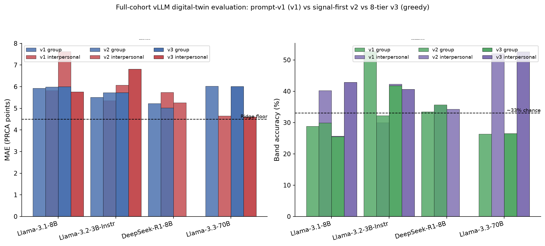{#fig-vllm-v1-cross fig-alt="Grouped grayscale bar charts comparing pooled mean absolute error and band accuracy across Llama-3.1-8B, Llama-3.2-3B, DeepSeek-R1-Distill-8B, and Llama-3.3-70B under prompt versions v1, v2, and v3."}
@fig-vllm-v1-cross is the manuscript’s primary live-result figure: pooled MAE / band accuracy for Llama-3.1-8B, Llama-3.2-3B, DeepSeek-R1-Distill-8B, and Llama-3.3-70B under prompt-`v1` and the GPU-evaluated `v2`/`v3` packages. **None** is a high-fidelity twin (exact match single-digit). Among non-collapsed runs, **DeepSeek** wins pooled group MAE (**5.22**) and is the most tier-stable; **Llama-3.2-3B** wins interpersonal MAE (**5.35**) and group band accuracy (**52.7%**); **Llama-3.1-8B** recovers interpersonal bands early (~52% at demos/geo) then **collapses at transit** (IP MAE 4.67 → **8.17**); **Llama-3.3-70B** is a mode-collapse cautionary case (≈93% constant prior `(18, 12)`).
| Model | MAE group ↓ | MAE IP ↓ | Exact G | Exact IP | Band G | Band IP | Notes |
|---|---:|---:|---:|---:|---:|---:|---|
| Llama-3.1-8B-Instruct | 5.92 | 5.82 | 6.1% | 9.0% | 28.8% | **40.2%** | Transit IP disaster |
| Llama-3.2-3B-Instruct | **5.51** | **5.35** | **9.1%** | 7.7% | **52.7%** | 30.0% | Best group bands |
| **DeepSeek-R1-Distill-Llama-8B** | **5.22** | 5.73 | 6.2% | 5.9% | 33.4% | 35.4% | Best group MAE; tier-stable |
| Llama-3.3-70B-Instruct | 6.02 | 4.65† | 6.4% | 12.4% | 26.3% | 52.0%† | †Constant prior; not person-tracking |
: Head-to-head pooled metrics across all prompt-`v1` tiers. {#tbl-v1-headtohead}
Non-collapsed models remain **above** the tabular Ridge floor (group MAE 4.49).
### RQ1–RQ3 pattern by model
| RQ | Llama-3.1-8B | Llama-3.2-3B | DeepSeek-R1-Distill-8B | Llama-3.3-70B |
|---|---|---|---|---|
| **RQ1 employment** | *Negligible* | *Negligible* | *Negligible* / slight IP help | *Null* (collapsed) |
| **RQ2 transit** | Group slight help; **IP disaster** | Small group help; IP worse | *Flat*; no IP collapse | *Null* (flat collapse) |
| **RQ3 full** | Group band up; IP worse than demos | Best group MAE (5.29); IP mixed | Best IP MAE at full (**5.42**) | *Negligible* dips only |
: Qualitative RQ1–RQ3 response pattern per model. {#tbl-rq-pattern}
**Interpretation.** Prompt-v1 transit text is a **model-dependent hazard**, not a universal aid. Prefer DeepSeek for group MAE, Llama-3.2 for group bands / IP MAE, treat Llama-3.1 as the cautionary transit-IP baseline that motivated packaging `v2`/`v3` (now GPU-evaluated below), and treat Llama-3.3-70B as a **mode-collapse** case. No model closes the gap to classical ML (~4.5 MAE).
Formal pages: [`docs/llm_baseline_llama31_v1.md`](docs/llm_baseline_llama31_v1.md) · [`docs/llm_baseline_llama32_instruct_v1.md`](docs/llm_baseline_llama32_instruct_v1.md) · [`docs/llm_baseline_deepseek_r1_distill_v1.md`](docs/llm_baseline_deepseek_r1_distill_v1.md) · [`docs/llm_baseline_llama33_70b_v1.md`](docs/llm_baseline_llama33_70b_v1.md). Memos: [`memos/vllm_v1_cross_model_comparison.qmd`](memos/vllm_v1_cross_model_comparison.qmd) · [`docs/llm_vllm_memo_agenda.md`](docs/llm_vllm_memo_agenda.md).
### `v2` results (signal-first packaging, `v2_enhanced` decode)
Prompt-`v2` keeps the five-tier topology with signal-first packaging (1-decimal geo, skipped Q27/Q29 when Never, independent group/IP subscale ask, mobility anti-bleed system text) and `v2_enhanced` decoding (temp 0.3, seed 42, guided JSON). Three models were GPU-evaluated (241 × 5 = 1,205 prompts each; `exports/v2/`):
| Model | MAE group ↓ | MAE IP ↓ | Band G | Band IP | Transit IP | Verdict vs v1 |
|---|---|---:|---:|---:|---:|---:|---|
| **DeepSeek-R1-Distill-Llama-8B** | **5.02** | **5.26** | 35.7% | 34.2% | **5.09** | **Improved both subscales; no IP collapse** |
| Llama-3.2-3B-Instruct | 5.73 | 6.07 | 32.2% | 42.3% | 5.77 | IP worse than v1 (5.35); no collapse |
| Llama-3.1-8B-Instruct | 5.99 | 7.63 | 29.9% | 25.7% | 8.23 | **IP collapse persists; base IP worse (demos 4.67 → 8.45)** |
: Pooled v2 metrics across the five tiers. {#tbl-v2-pooled}
DeepSeek v2 is the **best live result in the project** (group MAE **5.02**, below its v1 5.22 and the 3B/8B families) and stays flat at transit (IP 5.09, signed error near zero). Llama-3.2-3B’s v1 interpersonal win does **not** replicate under `v2` packaging/decode (pooled IP 5.35 → 6.07). For Llama-3.1, signal-first packaging and the mobility anti-bleed clause do **not** stop the transit collapse (transit IP 8.23 ≈ v1 8.17), and the independent-subscale ask shifts its *base* interpersonal calibration (demos IP 4.67 → **8.45**). Packaging therefore changes error patterns in **model-specific** directions — it is not a universal cure.
### `v3` results (8-tier ablation, greedy decode)
Prompt-`v3` adds three parallel single-cue tiers on the demos→employment→geo base — `v3_rideshare` (Q28 only), `v3_public_transit` (Q26 only), `v3_voice` (Q18.1/Q19 only) — for eight tiers per model (241 × 8 = 1,928 prompts). Three models were GPU-evaluated under greedy decode (`exports/v3/`; identical predictions to the `prior_v3_greedy` archives):
| Model | MAE group ↓ | MAE IP ↓ | Band G | Band IP | Parse | Notes |
|---|---|---:|---:|---:|---:|---:|---|
| Llama-3.1-8B-Instruct | 5.99 | 5.76 | 25.5% | **42.9%** | 100% | **Transit tier still collapses (IP 7.77); ablations stable** |
| Llama-3.2-3B-Instruct | 5.72 | 6.81 | 41.8% | 40.6% | 100% | IP worse than v1 (5.35) under `v3` packaging |
| Llama-3.3-70B-Instruct | 6.01 | 4.61† | 26.5% | 52.6%† | 100% | †Constant prior `(18, 12)` persists — not person-tracking |
: Pooled v3 metrics across all eight tiers. {#tbl-v3-pooled}
The 8-tier pooling mixes the collapsed `transit`/`full` tiers with stable ablations, so pooled IP is pulled back toward v1 (5.76). Llama-3.2-3B base remained a 0% JSON parse (as in v1) and is excluded.
For Llama-3.1, the ablations isolate the trigger precisely (IP MAE): `transit` bundle **7.77** vs `v3_public_transit` (Q26 only) **4.85**, `v3_voice` (Q18.1/Q19 only) **5.82**, `v3_rideshare` (Q28 only) **5.92**, and the geo base **4.63**. **No single cue collapses Llama-3.1's interpersonal recovery — only the bundled mobility dump does.** On group MAE, `v3_rideshare` (5.86) beats the kitchen-sink `transit` tier (6.07), aligning with the tabular `Q28`-dominance result. `v3_public_transit` (6.04) and `v3_voice` (5.64) group MAE stay near geo base (6.02).
:::{.callout-important}
## Llama-3.1 interpersonal collapse at `transit`
The most dramatic live finding is Llama-3.1-8B-Instruct’s interpersonal trajectory: IP MAE moves from **4.67** at `demos` to **8.17** at `transit` (+3.51), while band accuracy falls **51.9% → 15.4%** (−36.5 percentage points). This is not symmetric noise. Signed mean error (predicted − ground truth) flips from **−2.21** (under-prediction at demos) to **+6.52** at transit — systematic **over-prediction toward high interpersonal CA** once mobility cues appear [@santurkar2023]. The `full` tier partially walks back the damage (IP MAE **6.92**; signed error **+2.52**) but remains worse than demos-only. Group MAE, by contrast, improves slightly at transit (6.05 → 5.68).
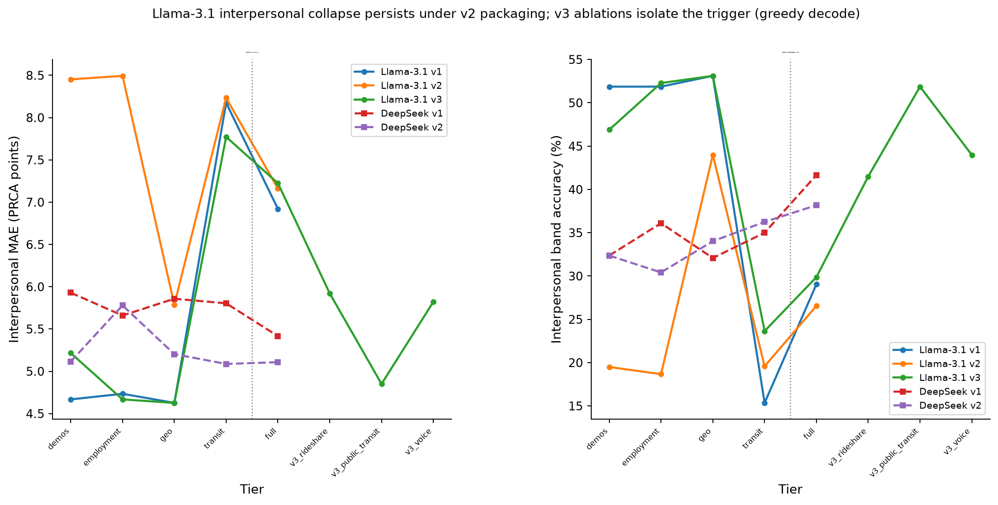{#fig-llama31-ip-collapse fig-alt="Line chart comparing interpersonal mean absolute error by persona tier for Llama-3.1-8B and DeepSeek-R1-Distill-8B across prompt versions v1, v2, and v3, showing Llama-3.1's collapse at the transit tier."}
@fig-llama31-ip-collapse contrasts Llama-3.1 with **DeepSeek-R1-Distill-Llama-8B** on the published per-tier summaries across prompt versions. DeepSeek’s IP MAE stays flat in v1 and improves under v2 (transit IP 5.09, signed error near zero), so the collapse is **model-specific**, not an inevitable property of adding transit text. Participant-level prediction histograms would require the gitignored raw vLLM export (`data/vllm/`); this revision uses the published tier aggregates in [`docs/llm_baseline_llama31_v1.md`](docs/llm_baseline_llama31_v1.md).
**What the model appears to be doing.** With only demos/employment/geo, Llama-3.1 behaves like a coarse interpersonal-band classifier (~52–53% band accuracy). Injecting the prompt-`v1` mobility dump (frequency, rides-per-day even when Never, ride-share, car) appears to activate a **high-anxiety stereotype prior** for interpersonal conversation — consistent with treating transit exposure as a social-threat cue rather than tracking individual scores. That failure mode motivated signal-first packaging (v2) and the `v3_rideshare` / `v3_public_transit` / `v3_voice` ablations ([`docs/persona_prompt_efficiency.md`](docs/persona_prompt_efficiency.md)), and the archived GPU runs now adjudicate it: **`v2` packaging does not stop the collapse** (transit IP 8.23 ≈ v1 8.17; base demos IP worsens to 8.45), while the **`v3` greedy ablations isolate the trigger** — single cues are stable (`v3_public_transit` IP 4.85, `v3_voice` 5.82, `v3_rideshare` 5.92) and only the bundled mobility dump collapses IP (7.77).
:::
## RQ3 / `full` tier and voice text
The `full` tier appends free-response Qualtrics items — **Q18.1** (advice for a nervous communicator) and **Q19** (ideal way to get around the city) — on top of the transit bundle. Among live prompt-`v1` runs:
| Model | `full` group MAE | `full` IP MAE | Notable `full` effect vs demos |
|---|---:|---:|---|
| Llama-3.1-8B | 5.84 | 6.92 | Group band ↑ 25.7% → **37.8%**; IP still worse than demos |
| Llama-3.2-3B | **5.29** | 5.53 | Best group MAE of any 3B tier |
| DeepSeek-R1-Distill-8B | 5.40 | **5.42** | Best IP MAE of any DeepSeek tier |
| Llama-3.3-70B | *~flat* | *~flat* | Mode collapse; uninterpretable |
: `full`-tier performance by model among live prompt-`v1` runs. {#tbl-full-tier}
:::{.callout-warning}
So open-text voice is **not uniformly helpful**: it can improve coarse group-band recovery (Llama-3.1) or IP MAE (DeepSeek) while leaving Llama-3.1 interpersonal continuous error elevated.
:::
Structured mobility cues still dominate the RQ2 hazard story.
**Qualitative read of voice content.** Of *N* = 241 analytic participants in the committed Posit cohort table, **149** have non-empty `Q18_advice` / `Q19` (median lengths ≈ 147 / 127 characters). An anonymized thematic sample (no IDs):
| Theme | Example gist (paraphrased / lightly excerpted) |
|---|---|
| Confidence coaching | “Stand, talk, and act confident… the other person is likely feeling just as nervous.” |
| Nervousness reciprocity | “Chances are the other people are also paying attention to themselves… They’re not looking to judge you.” |
| Slow / formulate | “Take it slow… think before speaking so you won’t make a wrong first impression.” |
| Breath / join | “Take a deep breath… wait for an opportunity to join the conversation.” |
| Natural flow | “Take their time… let the conversation flow naturally.” |
| Transit affinity | Ideal mobility = CTA / bus / train in a dense city (“quick, easy and cheap”). |
| Car necessity | Prefer own vehicle when transit feels overcrowded or unreliable; autonomy of schedule. |
| Mixed micro-mobility | Walk for local feel; bus for short hops; Uber when far. |
: Thematic sample of free-response full-tier voice content. {#tbl-voice-themes}
These texts are **attitude and coping language**, not demographics. When the model receives them at `full`, it gets participant voice about anxiety and mobility ideals — richer than Age/Sex alone, but still far short of the respondent’s full PRCA item pattern. The `v3_voice` ablation (geo base + Q18.1/Q19 only, without the transit dump) now has a greedy-decode answer: for Llama-3.1 it yields group MAE **5.64** and IP MAE **5.82** — better than the kitchen-sink `transit` (6.07 / 7.77) and `full` tiers with **no** interpersonal penalty, though IP remains above the geo base (4.63). Open-text voice is therefore not the driver of the transit collapse; the bundled structured mobility dump is.
## ML versus live LLM on shared metrics (full-cohort vLLM)
The mock-LLM pipeline diagnostics rendered in earlier revisions are removed. Every table in this section is computed from the **committed full-cohort vLLM exports** (`exports/v1/`, `exports/v2/`, `exports/v3/`) and the **seeded tabular suite** (tables committed in `artifacts/posit_full_cohort/ml_vs_llm/`); no deterministic-mock predictions are reported. The best live agent is ****DeepSeek-R1-Distill-Llama-8B** under `v2` packaging** (pooled group MAE 5.02, IP 5.26); Random Forest (`random_forest`) is the classical reference. Full write-up: [`memos/feature_predictive_power_ml_llm.qmd`](memos/feature_predictive_power_ml_llm.qmd); head-to-head framing: [`docs/ml_vs_llm.md`](docs/ml_vs_llm.md).
### MAE and band F1 by tier
Mean of group + interpersonal targets (*F*1 = macro-averaged harmonic mean of precision and recall; table: `metrics_ml_llm.csv`):
| Tier | RF MAE ↓ | DeepSeek v2 MAE | RF macro-F1 ↑ | DeepSeek v2 macro-F1 | RF band acc | DeepSeek v2 band acc |
|---|---:|---:|---:|---:|---:|---:|
| demos | 5.47 | **5.08** | **0.314** | 0.272 | **0.367** | 0.342 |
| employment | **5.35** | 5.47 | **0.312** | 0.250 | **0.369** | 0.342 |
| geo | **4.75** | 5.05 | **0.386** | 0.281 | **0.452** | 0.349 |
| transit | **4.48** | 5.03 | **0.422** | 0.265 | **0.506** | 0.360 |
: RF versus DeepSeek v2 MAE and band metrics by persona tier. {#tbl-mae-band-tier}
RF improves **monotonically** as tiers accumulate (MAE 5.47 → 4.48; macro-F1 0.31 → 0.42; band accuracy 0.37 → 0.51). DeepSeek v2 does not: `employment` is its *worst* tier (5.47), `transit` (5.03) barely beats `demos` (5.08), and its band metrics are flat at ~0.25–0.36 — below RF at every tier (@fig-f1-ml-vs-llm). In variance terms, the best tabular learner explains only a small share of true CA: RF $R^2$ rises from ≈ −0.37/−0.31 at `demos` (group / interpersonal) to **0.06–0.10** at `transit` (RMSE 5.82 / 5.51; table: `metrics_ml_llm.csv`). Even at its richest tier the classical suite leaves the large majority of individual CA variance unexplained, which contextualizes both the modest *d* = −0.46 transit-group CA contrast above and the single-digit exact-match ceiling of the persona agents.
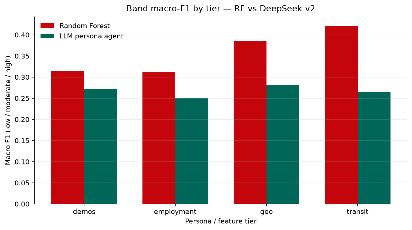{#fig-f1-ml-vs-llm fig-alt="Grouped grayscale bar chart comparing band macro-F1 by persona tier for Random Forest and DeepSeek v2 on group and interpersonal communication apprehension."}
### Who uses the information? Tier ablations
Incremental ΔMAE (Group CA) when each feature group is added (table: `tier_ablation.csv`):
| Step | RF ΔMAE | DeepSeek v2 ΔMAE |
|---|---:|---:|
| + employment | −0.12 | +0.10 |
| + geo | −0.55 | −0.26 |
| + transit | −0.37 | +0.08 |
: Incremental change in Group-CA MAE as each persona tier is added. {#tbl-tier-ablation}
The tabular learner converts each added covariate group into lower error; the LLM's profile is **non-monotonic** — employment and transit slightly *hurt* — matching its flat MAE across tiers and its higher `employment`-tier MAE above.
### What the estimated bands actually contain
When a model says “low / moderate / high”, which numeric scores did it emit, and how far are those from ground truth? Group CA, `transit` tier (table: `band_score_profile_ml_llm.csv`):
| Agent | Predicted band | *n* | Pred *M* (range) | GT *M* | MAE | Band precision |
|---|---:|---:|---:|---:|---:|---:|
| RF | low (6–13) | 96 | 11.95 (8.56–13.48) | 12.10 | 3.49 | 0.75 |
| RF | moderate (14–19) | 133 | 15.92 (13.50–19.47) | 16.30 | 5.31 | 0.31 |
| RF | high (20–30) | 12 | 21.12 (19.82–24.64) | 16.17 | 7.17 | 0.25 |
| DeepSeek v2 | low (6–13) | 78 | 11.18 (6–13) | 13.76 | 5.45 | 0.56 |
| DeepSeek v2 | moderate (14–19) | 162 | 15.01 (14–18) | 15.06 | 4.73 | 0.26 |
| DeepSeek v2 | high (20–30) | **0** | — | — | — | — |
: Predicted-score profiles inside each estimated band for Group CA at the transit tier. {#tbl-band-profiles}
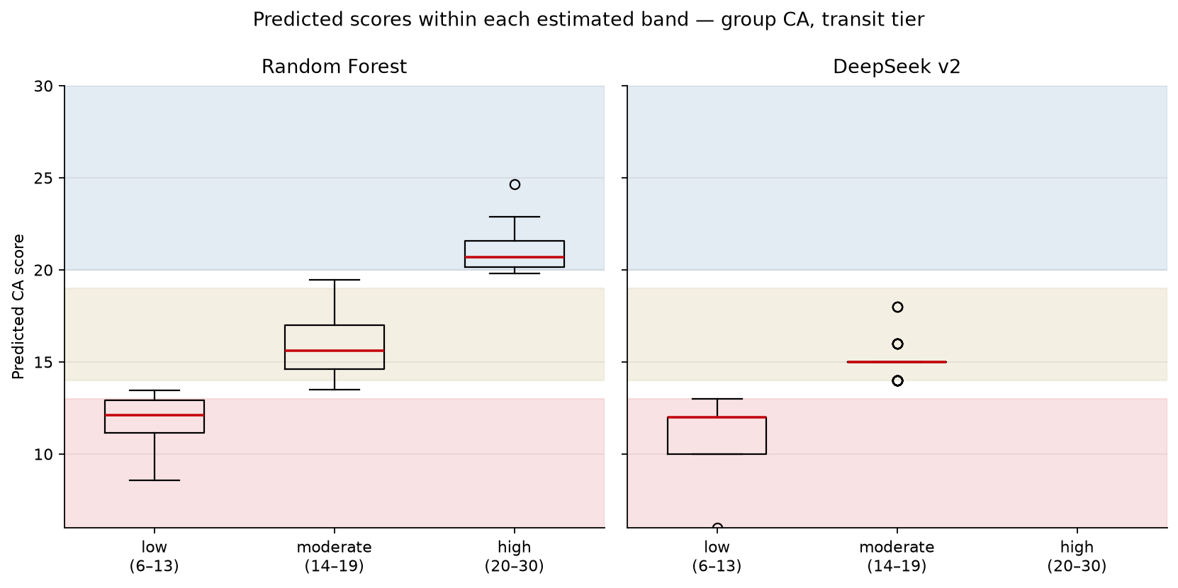{#fig-band-score-profiles fig-alt="Boxplots showing predicted score distributions within low, moderate, and high bands for Random Forest and DeepSeek v2 at the transit tier on group communication apprehension."}
:::{.callout-important}
Two quantification findings. **First, DeepSeek v2 never emits the high band for Group CA at `transit`** (0 of 240 predictions ≥ 20) — its “moderate” label absorbs every high-apprehension respondent (@fig-band-score-profiles). **Second, RF's rare high-band predictions (*n* = 12) are badly calibrated**: they land on respondents whose true mean is 16.17 (moderate), so RF precision on high is only 0.25. Both families are strong only on the low band.
:::
### Band discrimination: accuracy, distance, low-vs-high AUC
Disentangling MAE from discrimination: DeepSeek v2 is only ≈1.1× worse than RF on MAE, but on band separation it is much worse — its continuous scores do **not** rank apprehension (table: `band_discrimination_ml_llm.csv`).
| Agent | Tier | Side | Band acc | F1 macro | Mean band dist | AUC low-vs-high | Ordinal AUC |
|---|---:|---:|---:|---:|---:|---:|---:|
| RF | transit | Group | 0.481 | 0.386 | 0.573 | **0.717** | **0.650** |
| RF | transit | Interpersonal | 0.531 | 0.458 | 0.515 | **0.738** | **0.664** |
| DeepSeek v2 | transit | Group | 0.358 | 0.267 | 0.704 | 0.527 | 0.518 |
| DeepSeek v2 | transit | Interpersonal | 0.362 | 0.263 | 0.683 | 0.488 | 0.491 |
: Band discrimination at the `transit` tier: accuracy, distance, and AUC low-vs-high. {#tbl-band-discrimination}
*Notes.* AUC low-vs-high = predicted score separating ground-truth high (≥20) from low (≤13) respondents (moderates excluded); ordinal AUC = Hand–Till pairwise AUC over all three bands (0.5 = chance). Full per-tier/per-band table: `artifacts/posit_full_cohort/ml_vs_llm/band_discrimination_ml_llm.csv`.
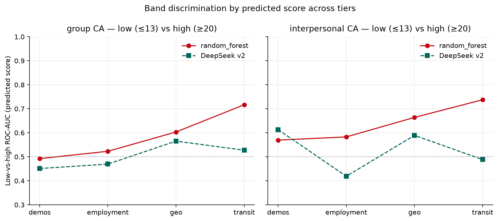{#fig-band-discrimination-auc fig-alt="Grouped grayscale bar chart comparing low-versus-high band ROC-AUC by persona tier for Random Forest and DeepSeek v2 on group and interpersonal communication apprehension, with a chance reference line at 0.50."}
:::{.callout-important}
RF's low-vs-high AUC climbs from ≈0.49 (`demos`) to **0.72–0.74** (`transit`); DeepSeek v2 stays near chance (0.45–0.53) at every tier (@fig-band-discrimination-auc). The LLM's error is **band-insensitive**: its scores hug the cohort mean, so absolute error is bounded while rank recovery fails. **MAE alone therefore understates the LLM's failure to recover the trait distribution** — band F1, band distance, and low-vs-high AUC belong alongside MAE in digital-twin evaluation.
:::
### Feature attributions: TreeSHAP on true CA vs SHAP on live LLM outputs
TreeSHAP mean \|SHAP| at the `transit` tier (predicting true Group CA) versus SHAP on the live LLM's outputs — an RF fit to DeepSeek v2's real vLLM predictions (surrogate $R^2 = 0.74$; tables: `shap_ml_group_raw.csv`, `shap_llm_surrogate_group_raw.csv`):
| Rank | RF → true CA | mean \|SHAP| | DeepSeek v2 output | mean \|SHAP| |
|---|---:|---:|---:|---:|
| 1 | Q28 (ride-share days) | 1.93 | LocationLatitude | 0.27 |
| 2 | Employment status | 0.83 | Age | 0.21 |
| 3 | Q26 (public-transit days) | 0.58 | LocationLongitude | 0.21 |
| 4 | LocationLatitude | 0.57 | Q28 | 0.19 |
| 5 | LocationLongitude | 0.54 | Country of residence | 0.15 |
| 6 | Age | 0.53 | Q26 | 0.15 |
: Top-six TreeSHAP attributions for true Group CA versus SHAP on DeepSeek v2's live outputs. {#tbl-shap-top6}
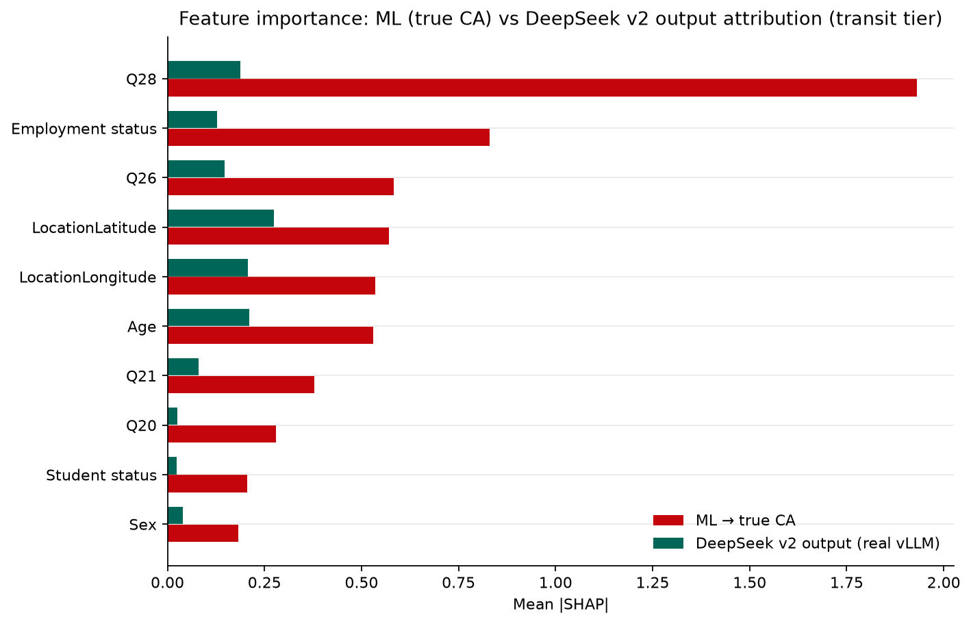{#fig-shap-ml-vs-llm fig-alt="Side-by-side horizontal bar charts comparing top mean absolute SHAP values for Random Forest predicting true group CA and a surrogate Random Forest fit to DeepSeek v2 live outputs at the transit tier."}
Ride-share days (Q28) and employment drive true-CA prediction, while the persona agent's live outputs are dominated by **geolocation and age** — over-weighting place/demographic cues relative to the mobility/employment mix that predicts the actual PRCA scores (@fig-shap-ml-vs-llm). Mean |SHAP| magnitudes are also approximately 7× smaller for the LLM output attribution, so no single profile feature dominates the agent's scores.
### Error by demographic group (live DeepSeek v2)
Before interpreting group-level error gaps, it is useful to anchor them against the ground-truth CA distribution per group (committed `ground_truth_aggregates.csv`; group-CA *M* (*SD*)):
```{python}
#| label: tbl-gt-demographic
#| tbl-cap: "Ground-Truth Group-CA by Demographic Slice (*N* = 241)"
#| tbl-colwidths: [30, 22, 22, 26]
gt_agg = pd.read_csv(COMMITTED_FULL / "ground_truth_aggregates.csv")
rows = []
for _, r in gt_agg[gt_agg["scope"].isin(["sex", "student_status", "employment"])].iterrows():
    label = r["group_key"] if str(r["group_key"]) != "nan" else "Student = Missing"
    rows.append(
        {
            "Slice": f"{label}",
            "n": f"{r['n']:.0f}",
            "Group CA *M* (*SD*)": f"{r['mean_group_ca']:.2f} ({r['std_group_ca']:.2f})",
            "Group band high (%)": f"{r['group_band_high_pct'] * 100:.1f}",
        }
    )
pd.DataFrame(rows)
```
*Note.* Group-CA means from the full matched analytic cohort. Full-time employment and (to a lesser degree) the student-status differences below sit at the floor of the "error by group" table that follows: they document the *true* group-level CA structure that the live agent's calibration split either tracks or misses.
Real stereotyping slices from the committed v2 export (`exports/v2/…/tables/stereotyping_by_*.csv`), group-CA MAE by tier:
| Group | demos | employment | geo | transit | n (transit) |
|---|---:|---:|---:|---:|---:|
| Student = Yes | 5.24 | 4.71 | 4.68 | 5.00 | 34 |
| Student = No | 5.07 | 5.23 | 4.95 | 4.89 | 190 |
| Female | 4.93 | 5.09 | 4.73 | 4.73 | 120 |
| Male | 5.17 | 5.21 | 5.04 | 5.20 | 120 |
| Full-Time | 4.37 | 4.63 | 4.35 | 4.39 | 148 |
| Part-Time | 6.06 | 5.84 | 6.00 | 5.55 | 31 |
| Other | 6.16 | 6.05 | 5.61 | 6.07 | 61 |
: Group-CA MAE by demographic slice across v2 tiers for **DeepSeek-R1-Distill-Llama-8B**. {#tbl-stereo-slices}
Sex and student-status MAE gaps are small (≤ ≈0.5 points). **Employment is the striking slice**: Full-Time error sits at 4.35–4.63 in every tier, while Part-Time and Other hover at 5.5–6.2. Signed error (predicted − true) is near zero for Full-Time (−0.01) but **−2.0 to −3.6 for Part-Time / Other** at every tier — the live agent systematically **under-predicts CA for non-full-time respondents** ([`docs/stereotyping_evaluation.md`](docs/stereotyping_evaluation.md)). The ground-truth slice above (Group CA *M* ≈ 13.3 for Full-Time vs ≈ 16.2 / 17.0 for Part-Time / Other; high-band prevalence ≈ 13% vs 26% / 37%) shows this is **not** symmetric noise: non-full-time respondents genuinely cluster higher on CA, so the agent's negative signed error is a real *calibration miss* on a subgroup with elevated trait levels, not just a scatter artifact. This sharpens the RQ1 story: employment does not *shrink* overall MAE, but it is a real **calibration split** in the live model.
## Secondary results: regular transit and mobility predictors
**Regular transit** is defined as `Q26` ∈ {`4-8 days a month`, `8 or more days a month`} (weekly-or-more), yielding **101 regular / 140 not regular** riders (prevalence = **0.419**) in the analytic cohort. The analyses below use stratified 5-fold Random Forests (`random_state=42`) unless noted. Full write-ups: [`memos/transit_riders_ca.qmd`](memos/transit_riders_ca.qmd), [`memos/geo_predicts_transit.qmd`](memos/geo_predicts_transit.qmd), [`memos/ca_scores_predict_transit.qmd`](memos/ca_scores_predict_transit.qmd), [`memos/q27_q28_predict_transit.qmd`](memos/q27_q28_predict_transit.qmd), [`memos/transit_covariate_followups.qmd`](memos/transit_covariate_followups.qmd).
### Regular riders differ in CA scores
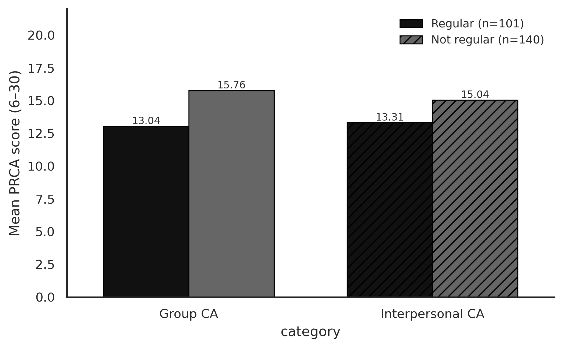
Welch tests on the matched cohort show lower CA among regular riders ([memo](memos/transit_riders_ca.qmd); @fig-transit-ca-means):
| Subscale | Regular *M* (*SD*) | Not regular *M* (*SD*) | Δ | Cohen's *d* | Welch *t* | *df* | *p* | 95% bootstrap CI for Δ |
|---|---:|---:|---:|---:|---:|---:|---:|---|
| Group CA | 13.04 (5.08) | 15.76 (6.42) | −2.72 | −0.46 | −3.68 | 236.91 | < .001 | [−4.15, −1.28] |
| Interpersonal CA | 13.31 (5.37) | 15.04 (6.04) | −1.73 | −0.30 | −2.34 | 228.80 | .020 | [−3.12, −0.25] |
: Welch contrasts for regular versus non-regular public-transit riders on PRCA subscales. {#tbl-welch}
*Note.* Cell sizes: *n* = 101 regular / 140 not regular.
```{python}
#| label: fig-transit-ca-means
#| fig-cap: "Mean Ground-Truth PRCA Scores for Regular Versus Non-Regular Public-Transit Riders"
#| fig-alt: "Grouped grayscale bar chart of mean group and interpersonal CA for regular and non-regular transit riders."
#| out-width: "75%"
g = secondary["transit_ca"]["group"]
i = secondary["transit_ca"]["interpersonal"]
fig, ax = plt.subplots(figsize=(6.4, 4.0))
grouped_bars(
    ax,
    ["Group CA", "Interpersonal CA"],
    {
        f"Regular (n={g['n_regular']})": [g["mean_regular"], i["mean_regular"]],
        f"Not regular (n={g['n_not_regular']})": [g["mean_not_regular"], i["mean_not_regular"]],
    },
    ylabel="Mean PRCA score (6–30)",
    ylim=(0, 22),
)
fig.tight_layout()
plt.show()
```
*Note.* Full matched analytic cohort. Means correspond to the Welch contrasts reported above and in [`memos/transit_riders_ca.qmd`](memos/transit_riders_ca.qmd).
### Geography and CA as classifiers of regular transit
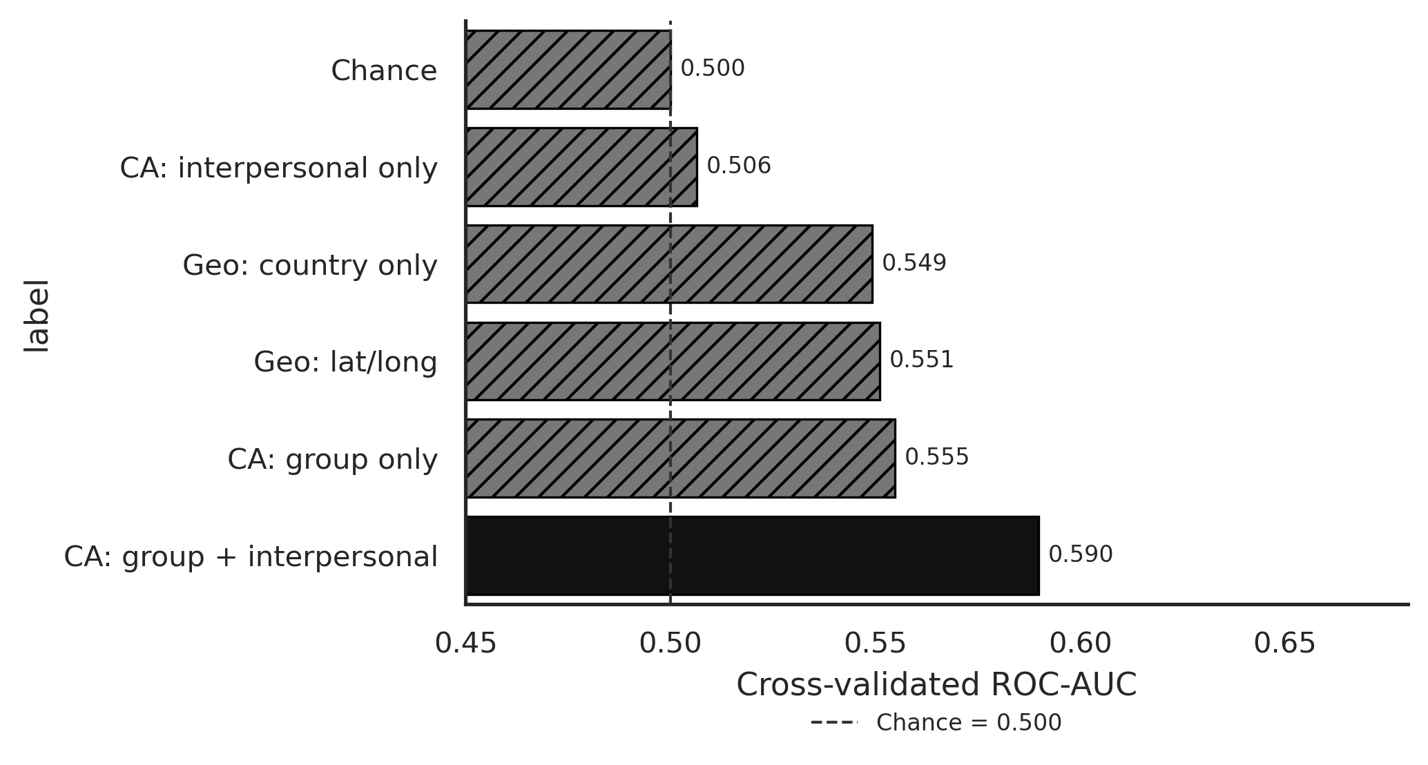
On the same outcome, a lat/long Random Forest yields cross-validated receiver-operating-characteristic AUC (CV ROC-AUC) = **0.551** (country-only AUC = **0.549**; chance = **0.500**; @fig-geo-ca-auc; [memo](memos/geo_predicts_transit.qmd)). A Random Forest on group + interpersonal CA yields CV ROC-AUC = **0.590** (group-only = **0.555**; interpersonal-only = **0.506**; out-of-fold confusion: true negatives = 76, false positives = 64, false negatives = 40, true positives = 61) ([memo](memos/ca_scores_predict_transit.qmd)).
```{python}
#| label: fig-geo-ca-auc
#| fig-cap: "Cross-Validated ROC-AUC for Geography and Communication-Apprehension Random Forests Predicting Regular Transit"
#| fig-alt: "Horizontal grayscale bar chart comparing ROC-AUC for lat/long, country-only, CA joint, CA ablations, and chance."
#| out-width: "85%"
labels = [
    "CA: group + interpersonal",
    "CA: group only",
    "Geo: lat/long",
    "Geo: country only",
    "CA: interpersonal only",
    "Chance",
]
vals = [
    secondary["ca_rf"]["roc_auc"],
    secondary["ca_rf"]["group_only"],
    secondary["geo_rf"]["roc_auc"],
    secondary["geo_rf"]["country_only_roc_auc"],
    secondary["ca_rf"]["interpersonal_only"],
    0.5,
]
fig, ax = plt.subplots(figsize=(7.0, 3.8))
horizontal_bars(
    ax,
    labels,
    vals,
    xlabel="Cross-validated ROC-AUC",
    highlight_index=0,
    vlines={"Chance = 0.500": 0.5},
    xlim=(0.45, 0.68),
    legend_loc="below",
)
fig.tight_layout()
plt.show()
```
*Note.* Stratified 5-fold CV, `random_state=42`, *N* = 241. Detailed results: [`memos/geo_predicts_transit.qmd`](memos/geo_predicts_transit.qmd); [`memos/ca_scores_predict_transit.qmd`](memos/ca_scores_predict_transit.qmd).
### Q27 and Q28 as traditional ML predictors of regular transit
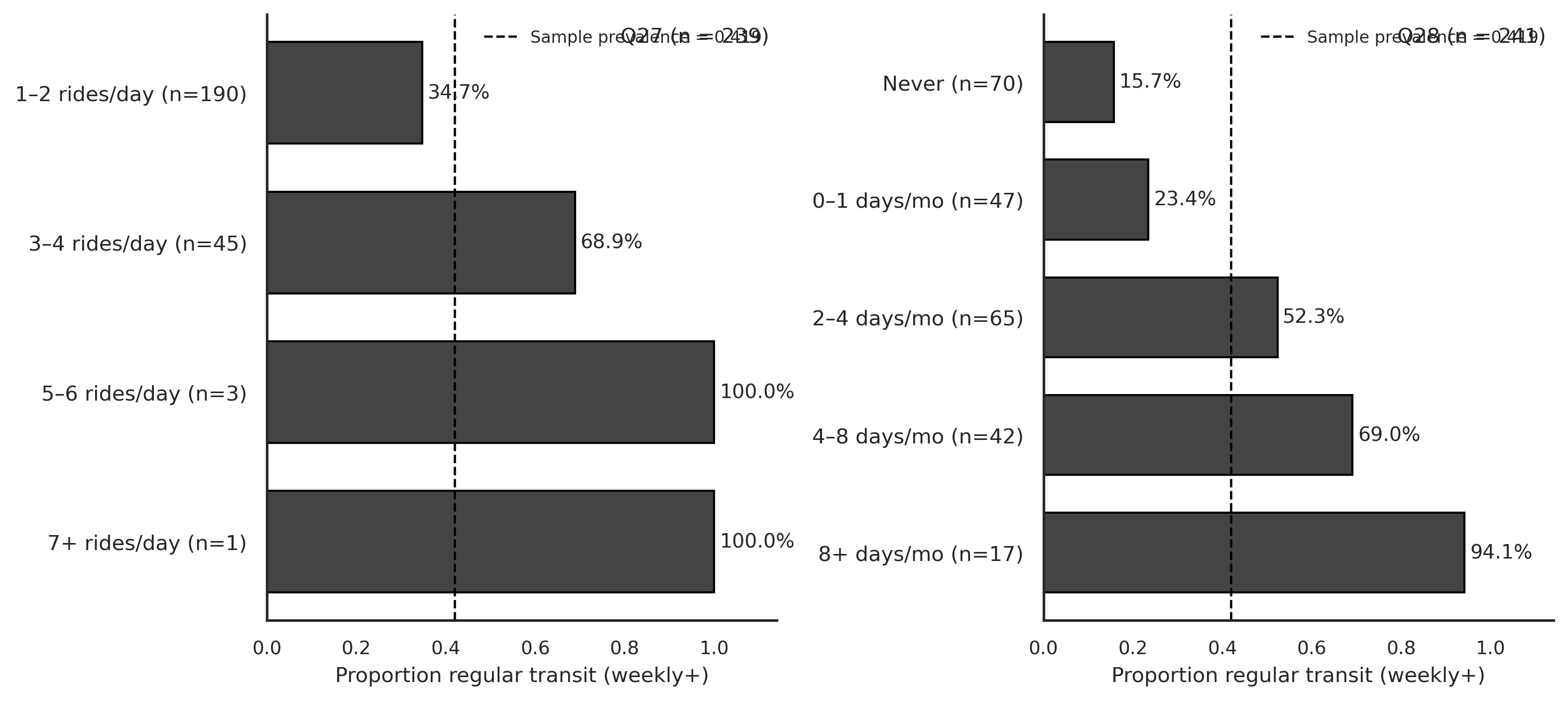
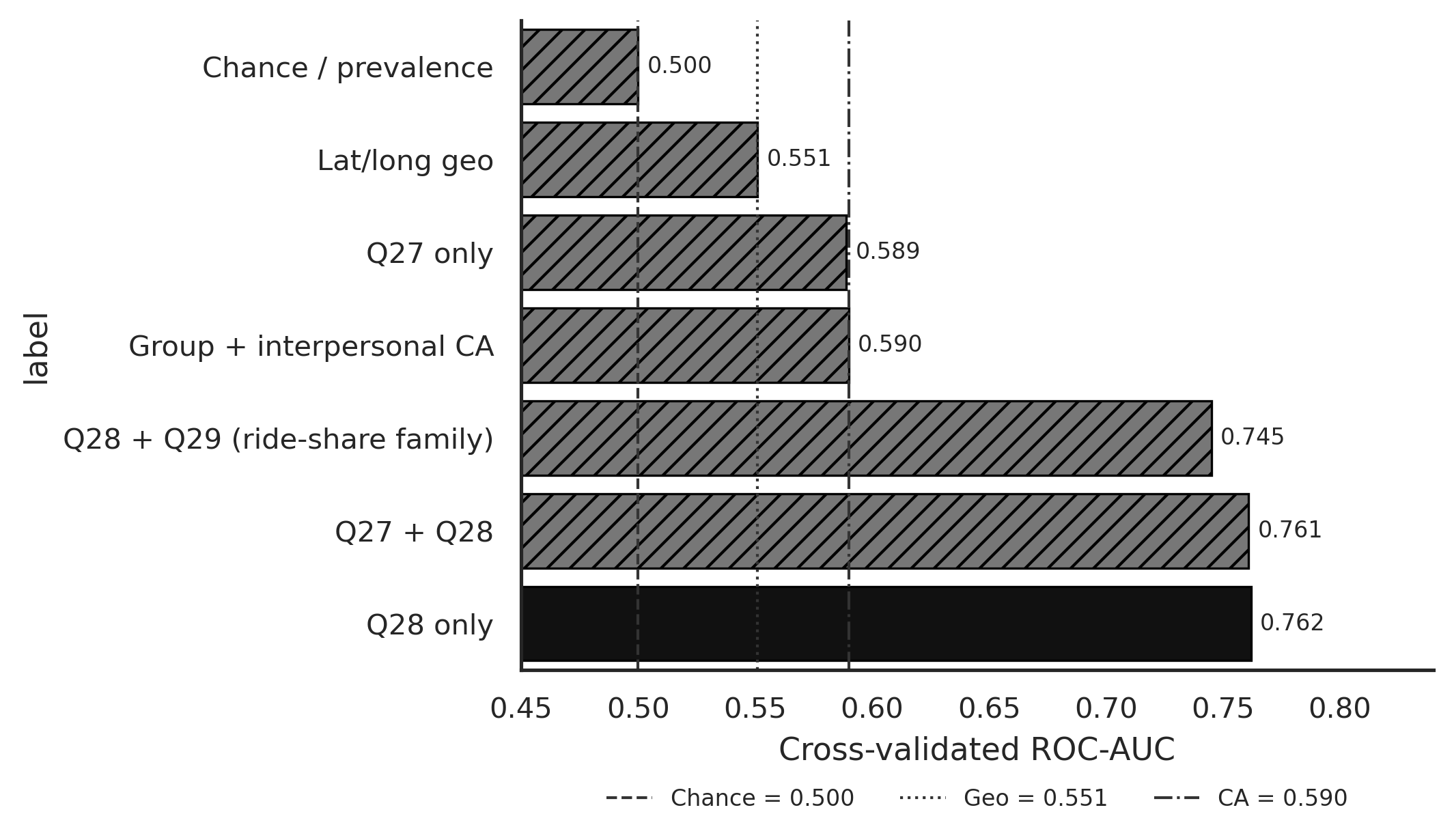
@fig-q27-q28-prev, @fig-q27-q28-auc, and @tbl-q27-q28-auc summarize the Q27/Q28 reverse-prediction results ([memo](memos/q27_q28_predict_transit.qmd)). **Q28** (ride-share days) shows a monotonic prevalence gradient from **15.7%** regular (Never) to **94.1%** regular (8+ days/month) and CV ROC-AUC = **0.762** (average precision [AP] = 0.689; balanced accuracy = 0.730; F1 = 0.702). **Q27** (rides on a typical transit day) yields CV ROC-AUC = **0.589**. The joint Q27+Q28 forest reaches AUC = **0.761** (Δ = −0.001 vs Q28 alone).
```{python}
#| label: fig-q27-q28-prev
#| fig-cap: "Proportion of Regular Transit Riders by Q27 Intensity and Q28 Ride-Share Days"
#| fig-alt: "Two-panel grayscale horizontal bar charts of regular-transit prevalence by Q27 and Q28 response levels."
#| out-width: "100%"
#| fig-dpi: 220
order27 = [
    "1-2 rides in a typical day",
    "3-4 rides in a typical day",
    "5-6 rides in a typical day",
    "7 or more rides in a typical day",
]
order28 = [
    "Never",
    "0-1 days a month",
    "2-4 days a month",
    "4-8 days a month",
    "8 or more days a month",
]
short27 = {
    "1-2 rides in a typical day": "1–2 rides/day",
    "3-4 rides in a typical day": "3–4 rides/day",
    "5-6 rides in a typical day": "5–6 rides/day",
    "7 or more rides in a typical day": "7+ rides/day",
}
short28 = {
    "Never": "Never",
    "0-1 days a month": "0–1 days/mo",
    "2-4 days a month": "2–4 days/mo",
    "4-8 days a month": "4–8 days/mo",
    "8 or more days a month": "8+ days/mo",
}
q27 = pd.DataFrame(secondary["q27_prevalence"])
q27["level"] = pd.Categorical(q27["level"], categories=order27, ordered=True)
q27 = q27.sort_values("level")
q28 = pd.DataFrame(secondary["q28_prevalence"])
q28["level"] = pd.Categorical(q28["level"], categories=order28, ordered=True)
q28 = q28.sort_values("level")

fig, axes = plt.subplots(1, 2, figsize=(10.6, 4.8))
for ax, frame, title, short_map in [
    (axes[0], q27, "Q27 (n = 239)", short27),
    (axes[1], q28, "Q28 (n = 241)", short28),
]:
    y = np.arange(len(frame))
    ax.barh(y, frame["prevalence"], color="#444444", edgecolor="black", height=0.68)
    ax.axvline(
        secondary["prevalence"],
        color="black",
        ls="--",
        lw=1.1,
        label=f"Sample prevalence = {secondary['prevalence']:.3f}",
    )
    ax.set_yticks(y)
    ax.set_yticklabels(
        [f"{short_map.get(lv, lv)} (n={int(n)})" for lv, n in zip(frame["level"], frame["n"])],
        fontsize=10,
    )
    ax.set_xlabel("Proportion regular transit (weekly+)", fontsize=10)
    ax.set_xlim(0, 1.14)
    for yi, v in zip(y, frame["prevalence"]):
        # Value labels always sit OUTSIDE the bar so they stay legible.
        ax.text(v + 0.012, yi, f"{v:.1%}", va="center", ha="left", fontsize=9.5)
    ax.invert_yaxis()
    apa_axes(ax)
    ax.tick_params(axis="x", labelsize=9)
    ax.text(0.985, 0.98, title, transform=ax.transAxes, ha="right", va="top", fontsize=10)
    ax.legend(frameon=False, fontsize=8, loc="upper right")
fig.tight_layout()
plt.show()
```
*Note.* Dashed line marks cohort prevalence (0.419). Cell sizes for Q27 levels above 3–4 rides are sparse (*n* = 3 and *n* = 1). Source memo: [`memos/q27_q28_predict_transit.qmd`](memos/q27_q28_predict_transit.qmd).
```{python}
#| label: tbl-q27-q28-auc
#| tbl-cap: "Cross-Validated Random Forest Performance for Q27, Q28, and Benchmarks"
cmp = pd.DataFrame(secondary["covariate_comparison"])
keep = [
    "q28_days",
    "q27_q28",
    "rideshare",
    "ca_benchmark",
    "q27_intensity",
    "geo_benchmark",
    "chance",
]
labels = {
    "q28_days": "Q28 only",
    "q27_q28": "Q27 + Q28",
    "rideshare": "Q28 + Q29 (ride-share family)",
    "ca_benchmark": "Group + interpersonal CA",
    "q27_intensity": "Q27 only",
    "geo_benchmark": "Lat/long geo",
    "chance": "Chance / prevalence",
}
tab = cmp[cmp["spec_key"].isin(keep)].copy()
tab["spec_key"] = pd.Categorical(tab["spec_key"], categories=keep, ordered=True)
tab = tab.sort_values("spec_key")
out = pd.DataFrame(
    {
        "Model": tab["spec_key"].map(labels),
        "n": tab["n"],
        "ROC-AUC": tab["roc_auc"],
        "Average precision": tab["average_precision"],
        "Balanced accuracy": tab["balanced_accuracy"],
        "F1": tab["f1"],
    }
)
out = out.round(
    {
        "ROC-AUC": 3,
        "Average precision": 3,
        "Balanced accuracy": 3,
        "F1": 3,
    }
)
out
```
```{python}
#| label: fig-q27-q28-auc
#| fig-cap: "Cross-Validated ROC-AUC for Q27, Q28, Joint, and Benchmark Models Predicting Regular Transit"
#| fig-alt: "Horizontal grayscale bar chart of ROC-AUC for Q28, Q27+Q28, rideshare family, CA, Q27, geo, and chance."
#| out-width: "90%"
plot_rows = out.dropna(subset=["ROC-AUC"]).copy()
fig, ax = plt.subplots(figsize=(7.2, 4.2))
horizontal_bars(
    ax,
    plot_rows["Model"].tolist(),
    plot_rows["ROC-AUC"].tolist(),
    xlabel="Cross-validated ROC-AUC",
    highlight_index=0,
    vlines={"Chance = 0.500": 0.5, "Geo = 0.551": 0.551, "CA = 0.590": 0.590},
    xlim=(0.45, 0.84),
    legend_loc="below",
)
fig.tight_layout()
plt.show()
```
*Note.* Stratified 5-fold CV, `random_state=42`. Q28 alone exceeds chance by +0.262 AUC, geography by +0.211, and CA scores by +0.172. Head-to-head mobility follow-ups (car access AUC = 0.607; employment AUC = 0.528; rideshare family AUC = 0.745) are in [`memos/transit_covariate_followups.qmd`](memos/transit_covariate_followups.qmd), [`memos/car_access_predicts_transit.qmd`](memos/car_access_predicts_transit.qmd), [`memos/employment_predicts_transit.qmd`](memos/employment_predicts_transit.qmd), and [`memos/rideshare_predicts_transit.qmd`](memos/rideshare_predicts_transit.qmd).
## Extended secondary results: wave-2 follow-up experiments
Wave-1 memos left concrete open questions (unused Prolific demographics; country vs coordinates; Q28 after car conditioning; psych vs mobility importance; country×car; Q27 within regular riders; fair common-*N* rankings; residual CA after Q28). Eight offline experiments address those gaps with the same matched cohort and RF / Welch toolkit (`ca-personas followup-experiments --seed 42`). The agenda and methods hub are [`docs/research_memo_agenda.md`](docs/research_memo_agenda.md) and [`docs/secondary_rq_followup_experiments.md`](docs/secondary_rq_followup_experiments.md).
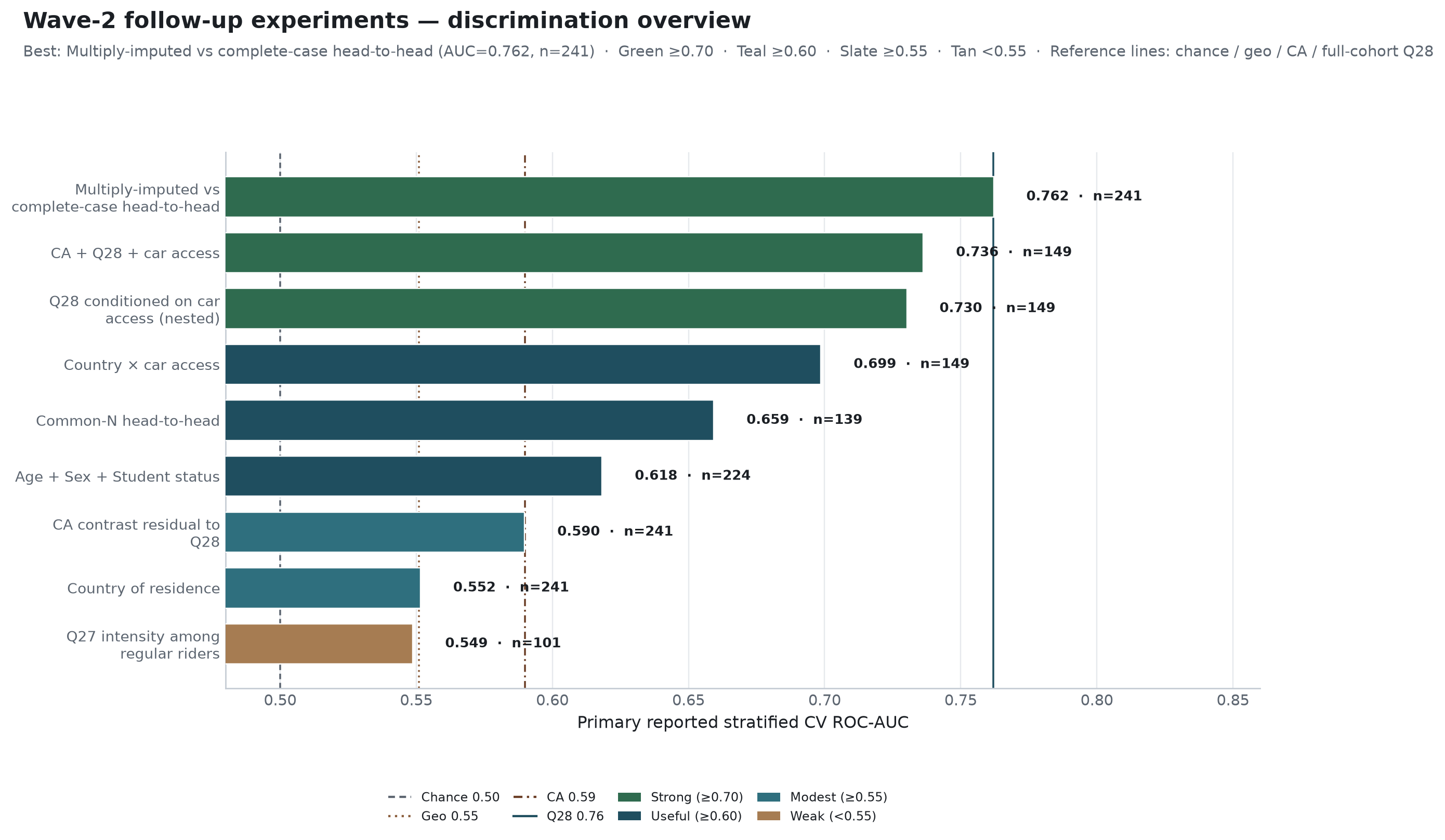{#fig-wave2-overview fig-alt="Horizontal bar chart of primary CV ROC-AUC for eight extended follow-up experiments with chance, geo, CA, and Q28 reference lines."}
### Overview of seeded results
| Experiment | Memo | *n* | ROC-AUC | Takeaway |
|---|---|---:|---:|---|
| CA + Q28 + car (joint) | [memo](memos/ca_mobility_joint_predicts_transit.qmd) | 149 | **0.736** | Mobility-dominated joint model |
| Q28 \| car (nested) | [memo](memos/q28_conditioned_on_car.qmd) | 149 | **0.730** | Q28 retains lift; car adds +0.066 AUC |
| Country + car | [memo](memos/country_car_predicts_transit.qmd) | 149 | **0.699** | Place × auto access synergy |
| Common-*N* best (Q28) | [memo](memos/common_n_head_to_head.qmd) | 139 | **0.659** | Rideshare ranking robust to equal *N* |
| Demographics (Age+Sex+Student) | [memo](memos/demographics_predict_transit.qmd) | 224 | **0.618** | Age-driven modest signal (younger 57.1% vs older 24.6% regular) |
| Residual CA (CA-only arm) | [memo](memos/residual_ca_after_rideshare.qmd) | 241 | **0.590** | CA-only AUC; joint CA+Q28 = 0.783 (+0.021 over Q28) |
| Country only | [memo](memos/country_predicts_transit.qmd) | 241 | **0.552** | Ties lat/long geo |
| Q27 intensity among riders | [memo](memos/q27_intensity_among_riders.qmd) | 95–101 | **0.549** | No useful within-rider classifier |
: Headline CV ROC-AUC for the eight wave-2 follow-up experiments. {#tbl-wave2-overview}
### Findings that change interpretation of the `transit` tier
1. **Q28 is not just “no car.”** On the car-complete overlap (*n* = 149), Q28 alone AUC = 0.665 and Q28+Q21 = 0.730—ride-share days retain discrimination after car conditioning, and car access adds +0.066 AUC ([nested memo](memos/q28_conditioned_on_car.qmd)).
2. **Fair rankings still crown rideshare.** Forcing Q28, car, country, geo, employment, CA, and demographics onto one complete-case frame (*n* = 139) preserves **Q28 > country > car > geo > employment ≈ CA ≈ demos** ([common-*N* memo](memos/common_n_head_to_head.qmd)).
3. **Demographics matter for bias audits.** Age+Sex+Student reach AUC = 0.618 on *n* = 224; younger tertiles are far more often weekly+ riders (57.1% vs 24.6% older). That is relevant to whether `demos`-tier LLM errors track age stereotyping ([demographics memo](memos/demographics_predict_transit.qmd)). Note this Age+Sex+Student feature set differs from the comprehensive-memo “demographics” ablation that also includes country (AUC = 0.636).
4. **CA is descriptively real, predictively redundant with Q28.** The overall regular-rider CA gap replicates (group Δ = −2.72, *d* = −0.46), but nesting CA with Q28 lifts AUC only from 0.762 → 0.783. Within Q28 strata the CA gap is heterogeneous—including a sign reversal in the 0–1 days cell ([residual CA memo](memos/residual_ca_after_rideshare.qmd)).
5. **Q27 remains weak even as an among-rider outcome.** High intensity among weekly+ riders is not recoverable from CA, Q28, car, employment, or demos (best AUC = 0.549).
6. **Kitchen-sink ceiling still looks like Q28.** A tuned comprehensive forest over demos + employment + geo + car + ride-share + CA reaches CV ROC-AUC = **0.824**, but permutation importance remains Q28-dominated ([comprehensive memo](memos/comprehensive_predictors_transit.qmd)).
## Unified results: one cohort, three question families
The primary (RQ1–RQ3), secondary (S1–S5), and focus (TF1–TF2) analyses share the same matched analytic cohort (*N* = 241) and the same information-tier logic, so they can be read as one measurement story. @tbl-unified collects each question's headline statistic and bottom line.
| Question | Headline result | Bottom line |
|---|---|---|
| RQ1 · employment | `v1` tier-level lift negligible; live DeepSeek v2 slice: Other MAE 6.07 vs Full-Time 4.39 at `transit` | Employment is a **calibration split**, not an error shrinker |
| RQ2 · transit | Model-dependent; Llama-3.1 IP collapse (+3.51 MAE; signed −2.21 → +6.52); DeepSeek flat | Bundled mobility cues are a hazard for some families |
| RQ3 · full voice | Best DeepSeek `full` IP 5.42; Llama-3.2 `full` group 5.29; v3 voice stable | Open-text voice helps some models, hurts others |
| S1 · transit ↔ CA | Regular riders lower CA (group Δ −2.72, *d* −0.46, *p* < .001) | CA and transit are descriptively related |
| S2 · geo → transit | lat/long RF CV AUC **0.551** (country 0.549) | Geography alone ≈ chance |
| S3 · CA → transit | CA RF CV AUC **0.590** (group 0.555, IP 0.506) | CA is a weak reverse predictor |
| S4 · Q27/Q28 → transit | Q28 AUC **0.762**; Q27 0.589; joint 0.761 | Ride-share exposure is the dominant mobility cue |
| S5 · covariate follow-ups | Q28 retains lift after car (0.730); CA+Q28+car 0.736; kitchen sink 0.824 | No covariate displaces Q28 |
| TF1 · profile → transit | Demos+employment+geo AUC **0.662** (0.672 with CA) | Ridership recoverable from non-mobility profile |
| TF2 · transit intensity | Q27 intensity AUC 0.549; MAE 1.22 vs majority 0.805 | Fine-grained intensity is not recoverable |
: Unified results across the primary, secondary, and focus question families. {#tbl-unified}
:::{.conclusion-block}
Three cross-cutting conclusions follow.
1. **The tabular signal is concentrated in mobility, and ride-share is its best proxy.** Q28 leads both predictive directions: it is the top TreeSHAP feature for true CA (mean \|SHAP| 1.93, more than twice the runner-up) and the top reverse predictor of weekly+ transit (AUC 0.762). Geography and CA scores stay near chance as reverse predictors (0.551 / 0.590); Q27 intensity and the TF2 intensity target remain weak. The persona tiers with the most justified information content are therefore `transit` (Q28/Q26) and `geo` — the same tiers that move RF error most (−0.55, −0.37 ΔMAE).
2. **The live LLM does not use that signal, and MAE alone hides how badly.** The best non-collapsed agent (DeepSeek v2) trails RF on every tier and metric, shows a non-monotonic tier profile (employment and transit slightly hurt), near-chance low-vs-high band discrimination (0.49–0.53 vs RF 0.72–0.74), no high-band emissions for group CA, and surrogate SHAP attributions dominated by geolocation/age rather than the Q28/employment mix that predicts true CA. Its absolute error is within ≈1.1× of ML — but only because its scores hug the cohort mean.
3. **Tier effects are not additive gifts; they are model- and target-dependent.** Employment is a calibration split in the live model (Part-Time/Other under-predicted by 2.0–3.6 points), transit breaks Llama-3.1's interpersonal recovery but not DeepSeek's, and voice text helps Llama-3.1's group bands while hurting its IP error. Reporting a single pooled MAE per model therefore obscures the patterned failures that matter for digital-twin evaluation; band F1, band distance, low-vs-high AUC, and group-level error slices are the load-bearing metrics.
:::
# Discussion
## Answers to the research questions
**RQ1 — employment.** Adding employment status does **not** shrink overall prediction error relative to `demos` (`v1` tier-level ΔMAE ≈ 0 across models), so we retain the null for the aggregate comparison. The alternative is nonetheless supported in a different form: live DeepSeek v2 shows a real **calibration split** — Full-Time respondents are under-approximated (MAE 4.35–4.63; signed error ≈ −0.01) while Part-Time/Other are systematically under-predicted (signed error −2.0 to −3.6) at every tier. Employment is therefore a *calibration split*, not an error shrinker. ([Memo: demographics → transit](memos/demographics_predict_transit.qmd) · [Memo: live-LLM stereotyping slices](memos/live_llm_stereotyping_slices.qmd))
**RQ2 — transit.** We reject the null for the LLM family in a *model-dependent* direction: the mobility bundle slightly helps Llama-3.1's group bands but produces a **transit-triggered interpersonal collapse** (IP MAE 4.67 → 8.17; signed error flips −2.21 → +6.52), while DeepSeek's IP error stays flat. `v3` greedy ablations isolate the trigger to the *bundled* mobility dump (bundled IP 7.77 vs single-cue 4.85–5.92). The classical RF baseline does improve monotonically with transit cues (MAE 5.47 → 4.48), so the null is rejected for the tabular family but the LLM uses mobility cues as stereotype proxies rather than psychologically sensible signal. ([Memo: Llama-3.1 v1 baseline](memos/vllm_v1_llama31_8b.qmd) · [Memo: `v2`/`v3` evaluation](memos/vllm_v2_v3_evaluation.qmd) · [Memo: cross-model comparison](memos/vllm_v1_cross_model_comparison.qmd))
**RQ3 — full voice.** We reject the null only for specific model–target pairs: DeepSeek's best `full` IP MAE (5.42), Llama-3.2's best `full` group MAE (5.29). For Llama-3.1, voice partially walks back the transit collapse (IP 8.17 → 6.92) but stays above demos. Open-text voice is **not uniformly helpful** — no consistent aggregate improvement. ([Memo: cross-model comparison](memos/vllm_v1_cross_model_comparison.qmd) · [Memo: `v2`/`v3` evaluation](memos/vllm_v2_v3_evaluation.qmd))
**S1 — transit ↔ CA.** We reject the null: regular riders report lower group (Δ = −2.72, *d* = −0.46, *p* < .001) and interpersonal (Δ = −1.73, *d* = −0.30, *p* = .020) CA. ([Memo: transit riders vs CA](memos/transit_riders_ca.qmd))
**S2 — geo → transit.** We retain the null: lat/long RF CV ROC-AUC = 0.551 (country 0.549), statistically ≈ chance. ([Memo: geography → transit](memos/geo_predicts_transit.qmd))
**S3 — CA → transit.** We retain the null in practical terms: CA RF ROC-AUC = 0.590, a weak reverse predictor well below conventional discriminability. ([Memo: CA → transit](memos/ca_scores_predict_transit.qmd))
**S4 — Q27/Q28 → transit.** We reject the null for ride-share: Q28 ROC-AUC = **0.762** (AP 0.689; F1 0.702). Q27 intensity alone is ≈ chance (0.589), and adding Q27 to Q28 adds nothing (0.761). ([Memo: Q27/Q28 → transit](memos/q27_q28_predict_transit.qmd))
**S5 — follow-ups.** We reject the null in a qualified form: wave-2 covariates add lift only when they extend the ride-share family (CA+Q28+car 0.736; kitchen sink 0.824), but no covariate displaces Q28's dominance. ([Memo: covariate follow-ups](memos/transit_covariate_followups.qmd) · [Memo: MI head-to-head](memos/mi_head_to_head.qmd))
**TF1 — profile → transit.** We reject the null: demos+employment+geo reaches AUC **0.662** (0.672 with CA) — ridership is partly recoverable from non-mobility profiles.
**TF2 — transit intensity.** We retain the null: fine-grained intensity is not recoverable (Q27 intensity AUC 0.549; Q26 ordinal MAE 1.22 vs majority 0.805). No answer is an answer here: transit frequency beyond weekly+ is effectively irreducible from the available covariates. ([TF1/TF2 memo](memos/transit_focus_regular_and_intensity.qmd))
## Primary digital-twin findings
On the full matched analytic cohort (*N* = 241), each participant yields five persona prompts (`demos` → `employment` → `geo` → `transit` → `full`) with fixed ground-truth PRCA scores. Full-cohort **prompt-`v1`** vLLM exports for four open-weight models show that none is a high-fidelity digital twin (exact match ≈6–9%), and all remain above the classical ML suite floor of **4.49** group MAE / **4.25** interpersonal MAE at `transit` ([`docs/ml_baselines.md`](docs/ml_baselines.md)). Among non-collapsed runs, **DeepSeek-R1-Distill-Llama-8B** minimizes pooled group MAE (**5.22**) with the most tier-stable profile; **Llama-3.2-3B-Instruct** leads interpersonal MAE (**5.35**) and group band accuracy (**52.7%**); **Llama-3.1-8B-Instruct** recovers interpersonal bands early but **collapses at transit** (IP MAE 4.67 → **8.17**); **Llama-3.3-70B** is a mode-collapse cautionary case, not a scale win ([`memos/vllm_v1_cross_model_comparison.qmd`](memos/vllm_v1_cross_model_comparison.qmd); @fig-vllm-v1-cross). Employment (RQ1) is negligible as a *tier-level* MAE mover across models, though the live DeepSeek v2 slices reveal a real **calibration split** (Part-Time/Other under-predicted by 2.0–3.6 points; see Results); transit text (RQ2) is a **model-dependent hazard** rather than a universal aid. The archived `v2`/`v3` exports refine this picture: DeepSeek improves under signal-first `v2` packaging (group MAE **5.02**, IP **5.26**, transit IP 5.09), while v2 does **not** fix Llama-3.1's collapse and even raises its base-tier IP error, and greedy `v3` ablations show the collapse is **combination-specific** (single-cue tiers 4.85–5.92; bundled dump 7.77).
## Why transit breaks Llama-3.1 but not DeepSeek
The Llama-3.1 interpersonal collapse is a signed-error flip (−2.21 → +6.52), not random scatter (@fig-llama31-ip-collapse). A plausible account — without claiming a causal architecture proof — is that **instruct-tuned** Llama-3.1 over-weights mobility language as a social-anxiety stereotype once the prompt-`v1` transit dump appears, whereas the **reasoning-distilled** DeepSeek sibling keeps IP MAE flat and signed error near zero at the same tier [@santurkar2023; @cheng2023]. This is consistent with the broader impersonation literature, in which the same persona-conditioned generation that recovers developmental or expertise effects simultaneously exposes systematic group biases [@salewski2023]. Training-data and decoding differences may also matter (DeepSeek’s post-`</think>` ingest still varied predictions; Llama-3.3-70B collapsed to a constant prior). The archived GPU runs add two causal clues. First, signal-first `v2` packaging with a mobility anti-bleed clause does **not** remove the failure (transit IP 8.23 ≈ v1 8.17) and shifts Llama-3.1's base interpersonal calibration (demos IP 4.67 → 8.45) — packaging is model-specific, not a universal cure, echoing findings that surface-level prompt formatting alone shifts model answers [@sclar2024]. Second, greedy `v3` single-cue ablations leave IP stable (`v3_public_transit` 4.85, `v3_voice` 5.82, `v3_rideshare` 5.92) while the bundled dump still collapses it (**7.77**) — the trigger is the **combination** of mobility cues in one transit bundle, not any single item ([`docs/persona_prompt_versions.qmd`](docs/persona_prompt_versions.qmd); [`docs/llm_v2_v3_enhanced_variants.md`](docs/llm_v2_v3_enhanced_variants.md)).
## Q28 dominance and persona design
Secondary analyses show that **Q28 ride-share days** dominate reverse prediction of weekly+ transit (AUC ≈ **0.762**) while geo and CA stay near chance and Q27 intensity is weak ([`memos/q27_q28_predict_transit.qmd`](memos/q27_q28_predict_transit.qmd)). Q28 is a **mobility exposure cue**, not a demographic label. For persona design that matters: stereotyping audits that slice only on Age/Sex/Student can miss bias that tracks ride-share or transit exposure [@cheng2023]. The evaluation battery therefore includes `regular_transit` and Q28 alongside Sex / Student / Employment / Age tertiles, reporting max−min MAE gaps and Δ-gap vs `demos` ([`docs/stereotyping_evaluation.md`](docs/stereotyping_evaluation.md)). Wave-2 follow-ups strengthen the Q28 claim — it retains lift after car access and leaves CA with only marginal incremental AUC ([`docs/secondary_rq_followup_experiments.md`](docs/secondary_rq_followup_experiments.md)). Treating ride-share as the high-value mobility tip (and isolating it in `v3_rideshare`) aligns persona prompts with the tabular importance ranking ([`docs/factor_feature_importance.md`](docs/factor_feature_importance.md)).
## Implications for survey research
Even the best live model (DeepSeek under `v2` packaging: group MAE **5.02**) remains roughly **1.1×** worse than Ridge regression on the same targets (~4.49), and exact twin recovery stays single-digit. That is a caution for **LLM-as-respondent / silicon-sampling** pipelines [@argyle2023; @park2024]: fluent persona inhabitance does not automatically recover individual psychometrics, parse success is not twin success (70B mode collapse), and classical tabular ceilings belong in the evaluation kit [@argyle2023; @hu2024]. Prompt packaging and model choice can change error *patterns* (transit hazard vs stability) without closing the ML gap. In the terms of the emerging LLM-simulation program — whether framed as *homo silicus* economic agents [@horton2023], cognitive-model finetuning [@binz2024], or the broader transformation of social-science research pipelines [@grossmann2023] — our benchmark adds a concrete psychometric caution: a model that is useful for *coarse opinion simulation* may still be a poor *individual-level digital twin* on a validated trait inventory, and the two claims must be separated. All displayed statistics on this page come from committed full-cohort vLLM exports, seeded tabular runs, and committed artifact tables — there are no mock-LLM claims; the deterministic mock provider is reserved for offline pipeline smoke tests.
:::{.callout-note}
## Limitations
Limitations include (a) same-wave observational designs for reverse-prediction AUCs, which cannot establish that ride-share causes weekly+ transit (or vice versa); (b) Prolific convenience-sample generalizability beyond the matched US-leaning online panel; (c) model and version drift — published numbers are pinned to specific Hugging Face checkpoints and the `20260726_*` / `20260728_*` / `20260729_*` / `20260730_*` export stamps; (d) keyless Cloud renders load committed full-cohort artifacts (vLLM export tables, seeded RF results, ML-vs-LLM metric tables) rather than re-running live inference, so a re-render does not refresh the exports; and (e) `v2`/`v3` GPU coverage is now broad but not complete — v2 is evaluated on Llama-3.1/3.2/DeepSeek and v3 (greedy) on Llama-3.1/3.2-3B-Instruct/3.3-70B, yet the canonical ``v3_enhanced`` decode refresh, a `v2`/`v3` run on the base 3B, and Llama-3.3-70B under the `large_model` preset remain pending, and the 8-tier v3 pooling mixes collapsed with stable tiers. Complete-case shrinkage for car-conditioned follow-ups further limits some wave-2 contrasts.
:::
## Future work
Priority GPU work is a **canonical v3 refresh under the ``v3_enhanced`` decode preset** (temp 0.3, seed 42, guided JSON, mobility anti-bleed system text) on Llama-3.1, DeepSeek, Llama-3.2, and Llama-3.3-70B, since the committed v3 packages are greedy-decode ablations (identical to the archived `prior_v3_greedy` runs). v2 coverage is complete except for the base 3B and 70B; DeepSeek v2 and the 8-tier greedy ablations are evaluated and reported above (`exports/v2/`, `exports/v3/`). Use `ca-personas stereotype-eval` on each live export so Sex/Age/Student/Employment **and** mobility-exposure MAE gaps are reported with tier-widening Δs ([`docs/llm_v2_v3_enhanced_variants.md`](docs/llm_v2_v3_enhanced_variants.md)). Additional follow-ups: constrained decoding for the 70B collapse (`large_model` preset), and participant-level prediction histograms once raw exports are staged.
## Conclusion
On a full matched Prolific↔Qualtrics cohort (*N* = 241), no open-weight persona agent came close to being a high-fidelity PRCA digital twin: every live model exceeded the classical suite floor, exact recovery stayed single-digit, and the best agent (DeepSeek under `v2` packaging, group MAE 5.02) trailed Ridge by roughly 1.1× while showing near-chance band discrimination and a systematic employment calibration split. The tabular story is starker and more interpretable — ride-share exposure (Q28) dominated prediction of weekly+ transit (AUC 0.762) and was the top feature for true CA, while geography, CA scores, and transit-day intensity added little. Together these findings argue that **persona prompting should be audited with band-level and attribution metrics, not MAE alone**, and that classical tabular learners remain the load-bearing benchmark for LLM-as-respondent claims. The memo scaffolding under [`memos/`](memos/README.md) and [`docs/`](docs/research_memo_agenda.md) documents each finding with the open questions that motivated the next wave of analyses.
# Reproducibility
```bash
python -m venv .venv
source .venv/bin/activate
pip install -r requirements.txt
pip install -e .
# Stage File A/B/C under ../sibling_data or CA_SIBLING_DATA=/tmp/sibling_data
ca-personas run --provider mock --join inner
ca-personas covariate-transit-rf --join inner --seed 42
python scripts/sync_posit_full_cohort_artifacts.py
python scripts/regenerate_ml_vs_llm_shap.py   # rebuild ML-vs-LLM tables/figures + artifact sync
quarto render
```
For **Posit Connect Cloud** [@quarto; @positconnect]: publish this repository [@psych755repo] with `_quarto.yml` as the primary file and `requirements.txt` present so Python dependencies install at build time. When private exports are absent, the manuscript loads committed full-cohort artifacts — participants, seeded secondary metrics, ML-vs-LLM metric tables (`artifacts/posit_full_cohort/ml_vs_llm/`), and the vLLM export tables including real stereotyping slices. From the project root, run [`./publish.sh`](publish.sh) (full analyses → render → Posit Connect publish) or `./publish.sh --skip-analysis --skip-render` to re-push the current `_site/`.
Source and author profile: [github.com/Exios66/psych755-jjb](https://github.com/Exios66/psych755-jjb) · [github.com/Exios66](https://github.com/Exios66) [@github].
# References
::: {#refs}
:::