Memo: Comprehensive predictors of regular transit
Research memorandum — kitchen-sink RF screen of survey covariates
Research question: Among available survey fields in the matched Prolific↔︎Qualtrics cohort (excluding the outcome source itself), which predictors most powerfully discriminate whether an individual takes public transportation regularly, and what ROC-AUC can a tuned Random Forest achieve?
1 Answer, Response, + Summary of Results
Using the Prolific↔︎Qualtrics matched cohort (File A + File B stacked joined to File C on Prolific ID / Q0; 252 matched rows; analytic n = 241 with complete PRCA items and non-missing Qualtrics geolocation), we screened demographics, employment, survey latitude/longitude, car access (Q20/Q21), ride-share behavior (Q28/Q29), and ground-truth PRCA scores ((McCroskey, 1970)) as predictors of regular public-transit use. Regular transit is defined as Q26 ∈ {4–8 days a month, 8 or more days a month} (weekly-or-more). Q26 was never used as a predictor. A mixed-type Random Forest ((Breiman, 2001); implemented via scikit-learn (Pedregosa et al., 2011)) (median/most-frequent imputation, one-hot encoding, stratified 5-fold CV) was tuned with RandomizedSearchCV to maximize ROC-AUC. Feature importance was assessed via univariate AUC, feature-group ablations, and original-column permutation importance.
Short answer: Yes—combining mobility-adjacent and demographic fields yields strong discrimination. The tuned kitchen-sink forest reaches CV ROC-AUC = 0.824 (default RF = 0.808; chance = 0.500). Ride-share frequency (Q28) is by far the dominant predictor, followed by car access (Q21) and age.
Figure Figure 1 shows permutation importance and the ROC curve for the tuned forest.
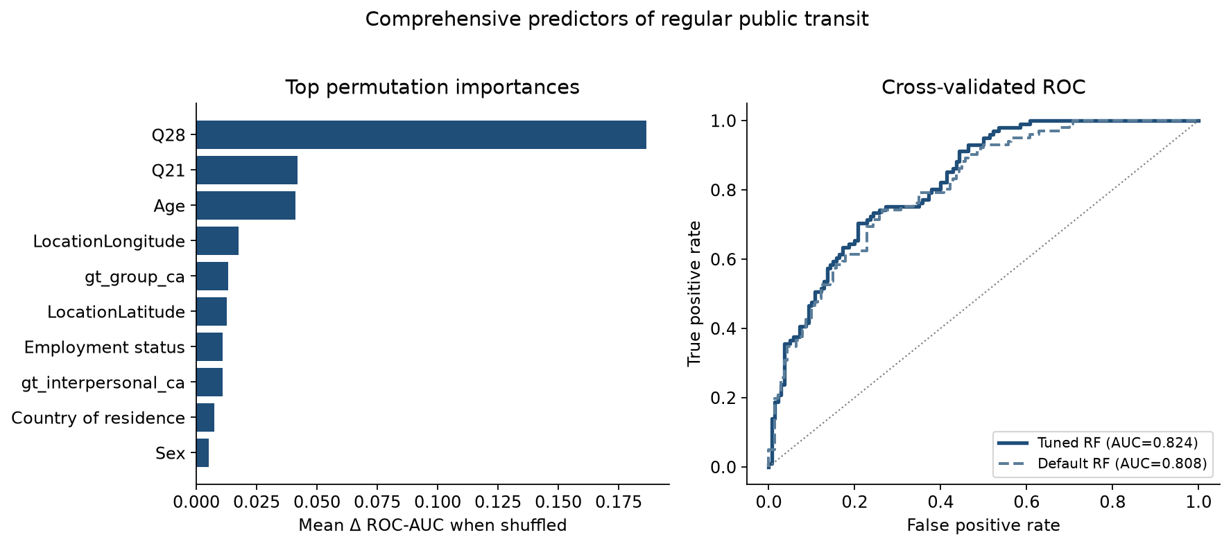
Univariate screen. Fit alone, Q28 already achieves AUC ≈ 0.762. No other primary feature exceeds 0.58 alone (Age ≈ 0.580; gt_group_ca ≈ 0.555; lat/lon and country ≈ 0.55). Proximal Q27 (rides on a typical public-transit day)—reserved for an upper-bound model—scores ≈ 0.594 univariate on the imputed n = 241 screen frame (cf. the seeded Q27-only model, AUC 0.589 on n = 239 in q27_q28_predict_transit.qmd).
Feature-group ablations. Table Table 1 reports the ablation comparisons.
| Model / comparison | ROC-AUC |
|---|---|
Rideshare group only (Q28, Q29) |
0.758 |
| Demographics only | 0.636 |
| CA scores only | 0.590 |
| Car access only | 0.563 |
| Geography only | 0.551 |
| Full kitchen sink (default RF) | 0.808 |
| Full kitchen sink (tuned RF) | 0.824 |
Upper bound (+ Q27) |
0.827 |
| Chance / prevalence | 0.500 |
Leave-one-group-out confirms the hierarchy: dropping rideshare costs ≈ −0.103 AUC; dropping car access ≈ −0.027; dropping CA ≈ −0.014. Dropping geography does not hurt (and can slightly help), indicating lat/lon add little once other fields are present.
Permutation importance (tuned model). Shuffling Q28 reduces ROC-AUC by ≈ ****0.187**** on average—several times larger than the next features (Q21 ≈ 0.042; Age ≈ 0.041; longitude ≈ 0.018; gt_group_ca ≈ 0.013). Best hyperparameters favored a relatively shallow forest (max_depth=4, max_features=log2, min_samples_leaf=2, class_weight=balanced).
Conclusion. In this cohort, regular public-transit use is most powerfully predicted by adjacent mobility behavior—especially ride-share days per month—augmented by car access and age. Communication apprehension and approximate geolocation remain detectable but secondary once mobility covariates are included. A tuned Random Forest over the defensible kitchen-sink feature set achieves strong out-of-fold discrimination (ROC-AUC ≈ 0.82). Adding proximal transit-intensity item Q27 yields only a marginal further lift, so the primary model already captures most available tabular signal without direct outcome leakage.
Sources: notebooks/secondary_rq_comprehensive_transit_rf.ipynb · src/ca_personas/comprehensive_transit_rf.py · ca-personas comprehensive-transit-rf · github.com/Exios66/psych755-jjb · formal write-up docs/secondary_rq_followup_experiments.md
2 What questions or uncertainties remain?
How much of the Q28 signal reflects a shared “multi-modal traveler” lifestyle versus a substitute/complement relationship with public transit? Would urban density, transit-access scores, or income—unavailable here—displace ride-share once included? Car/license items have substantial missingness (~38%); would complete automobility data reorder the importance ranking?
3 What other features may also well-predict regular public transit use?
City-level transit supply, commute distance, household vehicle count, and neighborhood density are natural next candidates. Within the present instrument, open-text mobility attitudes (Q19) and advice language (Q18.1) remain unused tabular/NLP features that could add signal beyond the structured kitchen sink.