Memo: Feature predictive power for CA (SHAP / F1)
Research memorandum — ML vs LLM attributions across persona tiers
Research question: Which demographic and behavioral features have the greatest predictive power for PRCA group and interpersonal communication-apprehension scores under traditional machine-learning models and LLM persona agents — as measured by SHAP attributions, band-level F1, and band discrimination (accuracy, distance, low-vs-high AUC)?
1 Answer, Response, + Summary of Results
Using the Prolific↔︎Qualtrics matched analytic cohort (File A + File B stacked joined to File C; 252 matched; analytic n = 241 with complete scorable PRCA items), we evaluated feature predictive power across the project’s cumulative information tiers (demos → employment → geo → transit). Traditional ML used cross-validated Random Forest ((Breiman, 2001); implemented via scikit-learn (Pedregosa et al., 2011)) and KNN regressors targeting ground-truth Group and Interpersonal CA (6–30). LLM persona agents ((Argyle et al., 2023)) were evaluated on the same tiers and metrics using the live vLLM exports — the best non-collapsed model, DeepSeek-R1-Distill-Llama-8B under prompt-v2 packaging (exports/v2/), replaces the earlier deterministic-mock stand-in. Attribution used TreeSHAP on RF models predicting true CA, plus surrogate SHAP on an RF fit to live LLM numeric outputs. Classification quality used macro / weighted / per-band F1, band accuracy, mean band distance, and low-vs-high ROC-AUC after mapping scores to classroom bands (low ≤13, moderate 14–19, high ≥20).
Full notebook: notebooks/feature_predictive_power_shap.ipynb · module ca_personas.shap_eval · real-export harness scripts/regenerate_ml_vs_llm_shap.py (the CLI ca-personas shap-eval --seed 42 keeps a deterministic mock for CI; this memo uses the committed vLLM exports).
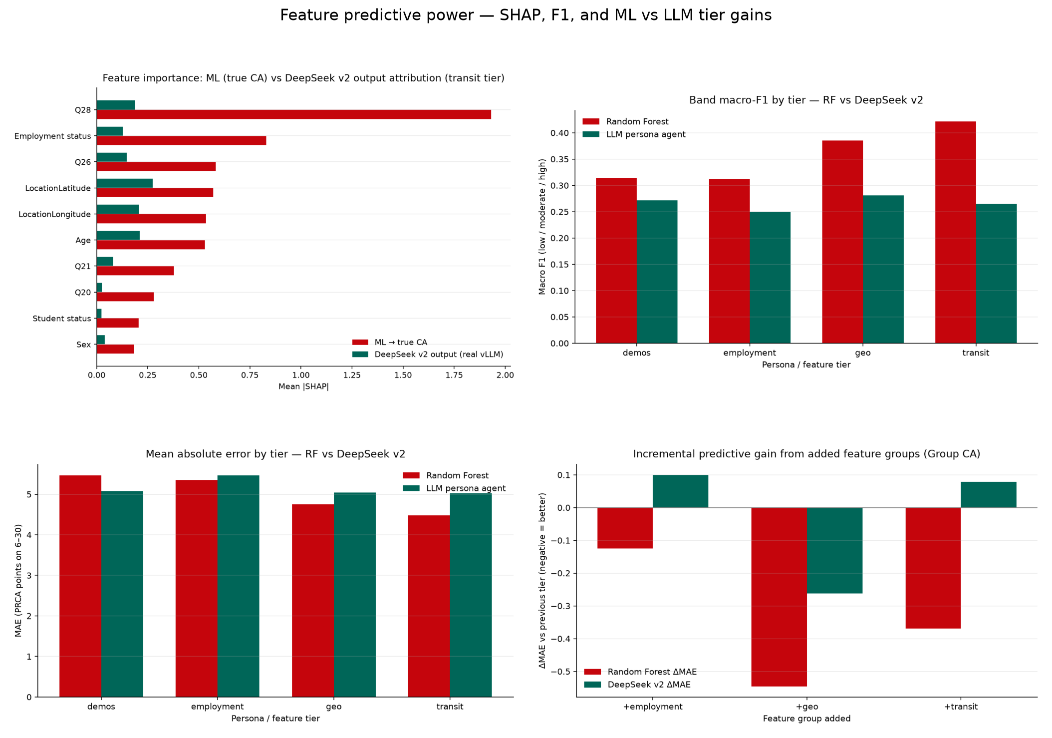
Short answer: Yes — structured covariates carry measurable predictive power for true CA under Random Forest, with ride-share frequency (Q28), employment status, public-transit frequency (Q26), and survey geolocation dominating TreeSHAP importance at the transit tier. Band macro-F1 rises from ~0.31 (demos) to ~0.42 (transit) for RF as information accumulates. The live LLM surrogate confirms the persona agent tracks profile features (surrogate \(R^2 \approx 0.74\) for Group CA), but the attribution profile is shifted: DeepSeek v2 over-weights geolocation and Age relative to the Q28/employment mix that predicts true CA, its low-vs-high band AUC is ≈ chance (0.53 group / 0.49 interpersonal at transit vs RF 0.72 / 0.74), it never emits the high-CA band (≥20), and it stays above the RF MAE floor at every tier (transit mean MAE 5.03 vs 4.48).
Figure Figure 1 summarizes the composite SHAP, F1/MAE-by-tier, and tier-ablation comparison.
1.1 Traditional ML — predictive power by tier
Mean metrics across Group + Interpersonal targets (random_state=42, stratified/K-fold CV). Note: the RF MAE column is the mean of group and interpersonal MAE from the classic RF+k-NN SHAP suite — not the group-only transit RF MAE (4.68) reported in docs/ml_baselines.md.
Table Table 1 reports the RF and KNN MAE and band-F1 metrics by tier.
| Tier | RF MAE ↓ (mean of both targets) | RF macro-F1 ↑ | RF band acc | KNN MAE | KNN macro-F1 |
|---|---|---|---|---|---|
| demos | 5.47 | 0.314 | 0.367 | 5.54 | 0.309 |
| employment | 5.35 | 0.312 | 0.369 | 5.54 | 0.334 |
| geo | 4.75 | 0.386 | 0.452 | 5.37 | 0.345 |
| transit | 4.48 | 0.422 | 0.506 | 4.98 | 0.372 |
At the transit tier, Group CA RF band F1 components were low=0.64 · moderate=0.42 · high=0.10 (macro=0.39); Interpersonal CA was stronger on high-band F1 (low=0.64 · moderate=0.48 · high=0.25; macro=0.46). Exact integer accuracy stayed low (~0.07), confirming that band-level metrics, not exact match, are the appropriate classification summary on a 6–30 scale.
Tier ablation (Group CA, RF). Adding geo cut MAE by −0.55 points vs employment; adding transit cut another −0.37, with corresponding macro-F1 gains (+0.05 then +0.03). Employment alone produced only a small MAE improvement over demos.
1.2 SHAP — features driving ML predictions of true CA
TreeSHAP mean \(\|SHAP\|\) (aggregated to raw fields) for RF → true Group CA at the transit tier (see Table Table 2). This ranking (predicting CA) is not interchangeable with the permutation ranking in docs/factor_feature_importance.md (predicting regular transit), where Age outranks employment.
| Rank | Feature | Mean \(\|SHAP\|\) |
|---|---|---|
| 1 | Q28 (ride-share days) |
1.93 |
| 2 | Employment status | 0.83 |
| 3 | Q26 (public-transit days) |
0.58 |
| 4 | LocationLatitude | 0.57 |
| 5 | LocationLongitude | 0.54 |
| 6 | Age | 0.53 |
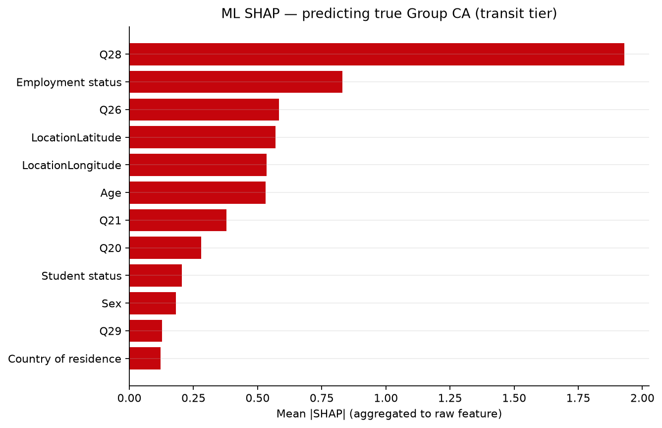
As shown in Figure Figure 2, transportation items and employment dominate over core demographics (Sex, Student status), supporting the primary research focus: RQ1–RQ2 covariates are not decorative — they reshape predicted apprehension under classical ML.
1.3 Live LLM persona agents — performance and surrogate SHAP
All LLM figures below use the committed vLLM exports (full cohort, N = 241 per tier), not the mock provider. The headline agent is DeepSeek v2 — the best non-collapsed live model (pooled group MAE 5.02, transit IP MAE 5.09); Llama-3.1’s interpersonal collapse at transit and Llama-3.2’s non-monotonic profile are reported in the manuscript and docs/llm_v2_v3_enhanced_variants.md.
Table Table 3 reports the tier-by-tier RF vs DeepSeek v2 MAE and band metrics.
| Tier | RF MAE ↓ | DeepSeek v2 MAE ↓ | RF macro-F1 ↑ | DeepSeek v2 macro-F1 | RF band acc | DeepSeek v2 band acc |
|---|---|---|---|---|---|---|
| demos | 5.47 | 5.08 | 0.314 | 0.272 | 0.367 | 0.342 |
| employment | 5.35 | 5.47 | 0.312 | 0.250 | 0.369 | 0.342 |
| geo | 4.75 | 5.05 | 0.386 | 0.281 | 0.452 | 0.349 |
| transit | 4.48 | 5.03 | 0.422 | 0.265 | 0.506 | 0.360 |
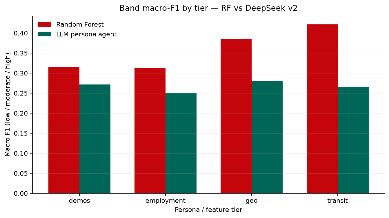
Mean of group + interpersonal targets. DeepSeek v2 trails RF on every tier and metric. Its tier profile is also flatter — employment and transit add nothing (and slightly worsen) LLM error, whereas RF improves monotonically with information.
Surrogate SHAP (RF predicting live LLM Group CA from tabular features; \(R^2 = 0.74\)) ranked lat/long, Age, Q28, country, Q26, employment highest — i.e., the persona agent’s outputs track place and age more than the Q28/employment mix that predicts true CA. Magnitudes are also compressed (0.13–0.27 vs ML’s 0.53–1.93), so no single profile feature dominates the agent’s scores (Table Table 4):
| Rank | DeepSeek v2 surrogate \(\|SHAP\|\) | RF \(\|SHAP\|\) (true CA) |
|---|---|---|
| 1 | LocationLatitude 0.27 | Q28 1.93 |
| 2 | Age 0.21 | Employment status 0.83 |
| 3 | LocationLongitude 0.21 | Q26 0.58 |
| 4 | Q28 0.19 |
LocationLatitude 0.57 |
| 5 | Country of residence 0.15 | LocationLongitude 0.54 |
| 6 | Q26 0.15 |
Age 0.53 |
| 7 | Employment status 0.13 | Q21 0.38 |
Figure Figure 3 juxtaposes the ML TreeSHAP and DeepSeek v2 surrogate SHAP bars.
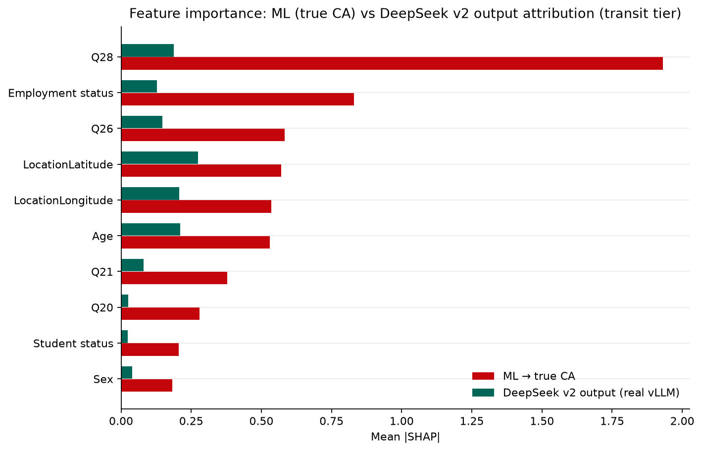
Figure Figure 4 plots band macro-F1 by tier for RF vs DeepSeek v2.
1.4 What the estimated bands actually contain
When a model says “low”, “moderate”, or “high”, which numeric scores did it output, and how do they relate to ground truth? Group CA, transit tier (Table Table 5):
| Agent | Predicted band | n | Pred score M (range) | GT score M | MAE | Band precision |
|---|---|---|---|---|---|---|
| RF | low (6–13) | 96 | 11.95 (8.56–13.48) | 12.10 | 3.49 | 0.75 |
| RF | moderate (14–19) | 133 | 15.92 (13.50–19.47) | 16.30 | 5.31 | 0.31 |
| RF | high (20–30) | 12 | 21.12 (19.82–24.64) | 16.17 | 7.17 | 0.25 |
| DeepSeek v2 | low (6–13) | 78 | 11.18 (6–13) | 13.76 | 5.45 | 0.56 |
| DeepSeek v2 | moderate (14–19) | 162 | 15.01 (14–18) | 15.06 | 4.73 | 0.26 |
| DeepSeek v2 | high (20–30) | 0 | — | — | — | — |
Figure Figure 5 shows the predicted-score profiles inside each estimated band.
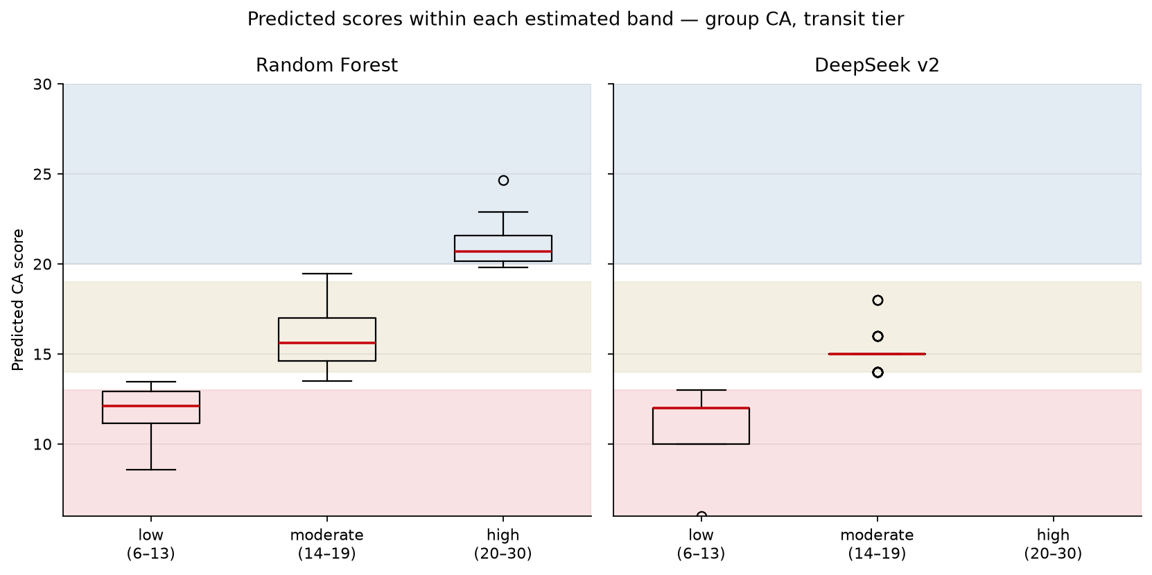
Two quantification findings stand out. First, the LLM never emits the high band for Group CA at transit (0 of 240 predictions ≥ 20; n = 3 at geo, all exactly 20.0) — its “moderate” label covers the full 14–18 span and absorbs every high-apprehension respondent. Second, RF’s rare high-band predictions (n = 12) are badly calibrated: they land on respondents whose true mean is 16.17 (moderate), so RF precision on high is only 0.25. Both families are strong only on the low band; band precision collapses to 0.26–0.31 on moderate/high.
1.5 Band discrimination (accuracy, distance, low-vs-high AUC)
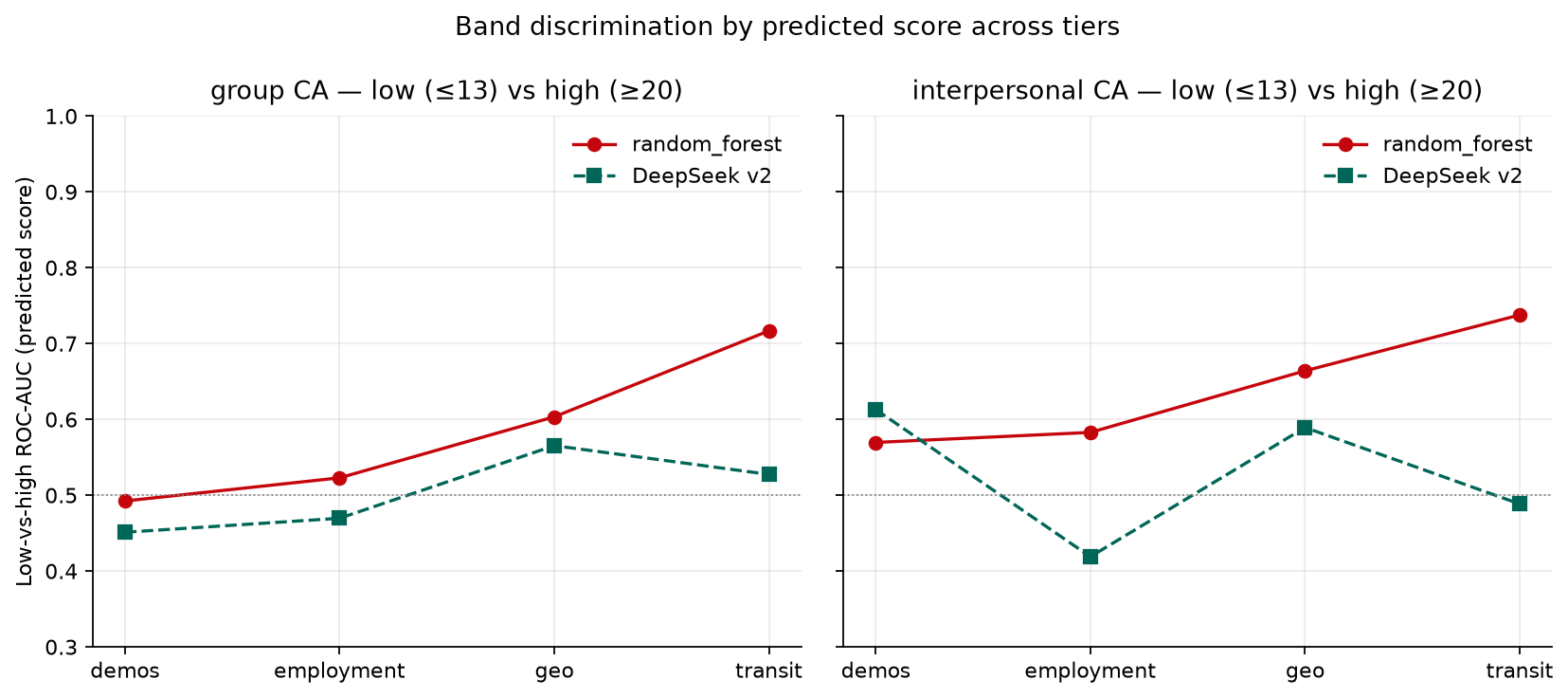
Disentangling MAE from discrimination: the LLM is only ~1.1× worse on MAE, but on band separation it is much worse — its continuous scores are effectively uninformative about low vs high apprehension (Table Table 6).
| Tier | Agent | Side | Band acc | F1 macro | Mean band dist | AUC low-vs-high | Ordinal AUC |
|---|---|---|---|---|---|---|---|
| transit | RF | Group | 0.481 | 0.386 | 0.573 | 0.717 | 0.650 |
| transit | RF | Interpersonal | 0.531 | 0.458 | 0.515 | 0.738 | 0.664 |
| transit | DeepSeek v2 | Group | 0.358 | 0.267 | 0.704 | 0.527 | 0.518 |
| transit | DeepSeek v2 | Interpersonal | 0.362 | 0.263 | 0.683 | 0.488 | 0.491 |
Notes. AUC low-vs-high = predicted score separating ground-truth high (≥20) from low (≤13) respondents (moderates excluded); ordinal AUC = Hand–Till pairwise AUC over all three bands (0.5 = chance). Full per-tier/per-band table: outputs/shap_eval/band_discrimination_ml_llm.csv.
Figure Figure 6 plots the low-vs-high ROC-AUC across tiers.
Figures Figure 7 and Figure 8 show the RF and DeepSeek v2 band confusion matrices.
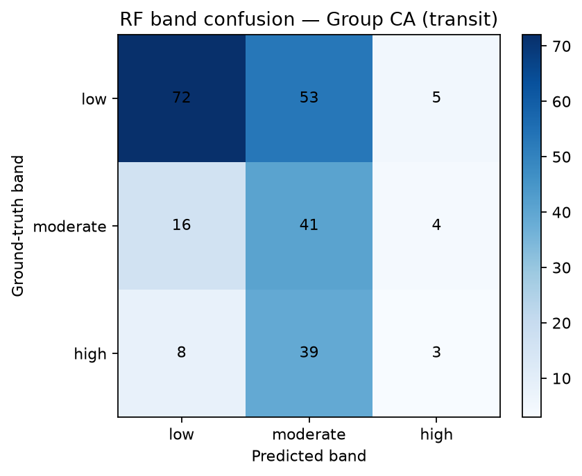
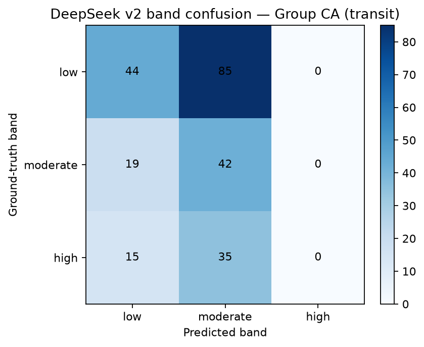
The discrimination gap widens as tiers accumulate: RF’s low-vs-high AUC climbs from ~0.49 (demos) to 0.72–0.74 (transit), while DeepSeek v2 stays at 0.49–0.53 across tiers (near chance). This is the mechanism behind the small MAE gap: the LLM is consistently near the cohort mean, so its absolute error is bounded, but its scores do not rank apprehension. Mean band distance tells the same story (RF 0.51–0.57 ≈ half a band off; DeepSeek v2 0.68–0.70). MAE alone therefore understates the LLM’s failure to recover the trait distribution.
Conclusion. Feature predictive power for communication apprehension in this matched cohort is real but moderate: richer tiers improve RF MAE, band F1, and low-vs-high discrimination, and TreeSHAP attributes that lift primarily to transit use, employment, and geolocation. The live LLM (DeepSeek v2) remains above the RF floor on every score and band metric, over-weights place/age in its surrogate attributions, avoids the high-CA band entirely, and shows near-chance band discrimination. LLM persona evaluation should therefore report band F1, band accuracy, band distance, and low-vs-high AUC alongside MAE, and use surrogate SHAP (or tier ablation) to audit whether the agent tracks the same covariates that predict true CA — or instead over-weights demographic/geographic stereotypes.
Sources: notebooks/feature_predictive_power_shap.ipynb · src/ca_personas/shap_eval.py · ca-personas shap-eval (mock for CI) · scripts/regenerate_ml_vs_llm_shap.py (real vLLM exports) · artifacts outputs/shap_eval/ (synced to artifacts/posit_full_cohort/ml_vs_llm/ for manuscript renders) · exports/v2/ · github.com/Exios66/psych755-jjb
2 What questions or uncertainties remain?
Does the canonical v3_enhanced decode (temp 0.3, guided JSON) change DeepSeek’s near-chance band discrimination, or is high-band avoidance intrinsic to the reasoning-distilled family? Would interaction SHAP (employment × transit) explain the residual over-weighting of place/age? Are band rankings stable under alternate cutoffs (e.g., ≤12 / ≥21)? Do the smaller Llama-3.2–3B and collapsed Llama-3.1/3.3–70B exports show the same discrimination floor or worse?
3 What other analyses pair with this memo?
Secondary RQs on transit↔︎CA mean differences and CA/geo → regular-transit Random Forests (transit_riders_ca.qmd, geo_predicts_transit.qmd) ask the reverse predictive direction. The present memo asks which inputs best recover CA under ML and LLM personification, and which bands the models actually separate. Live-model stereotyping slices on the same v2 export (live_llm_stereotyping_slices.qmd) and the cross-model / v2-v3 ranking memos (vllm_v1_cross_model_comparison.qmd, vllm_v2_v3_evaluation.qmd) complete the LLM-side picture.