Memo: Do Q27 and Q28 predict regular public transit?
Research memorandum — transit intensity & ride-share days in traditional ML
Research question: In traditional machine-learning classifiers, how much predictive power do survey items Q27 (rides on a typical public-transit day) and Q28 (ride-share days in the last three months) carry for regular public-transit use?
Companion memos: rideshare_predicts_transit.qmd · transit_covariate_followups.qmd · parent geo_predicts_transit.qmd
Manuscript: index.qmd § Secondary results: Q27/Q28 as ML predictors of regular transit
1 Answer, Response, + Summary of Results
Using the Prolific↔︎Qualtrics matched analytic cohort (File A + File B joined to File C; base n = 241 with complete PRCA and usable Q26), we define regular transit as Q26 ∈ {4–8 days a month, 8 or more days a month} (weekly-or-more). We then fit balanced ****Random Forests ((Breiman, 2001)) with stratified 5-fold CV (random_state=42) using categorical one-hot encodings of the survey items in Table Table 1:
Q27 and Q28 survey items.
| Item | Stem (abridged) | Role |
|---|---|---|
Q27 |
On a typical day of public transportation use, how many rides do you take? | Within-mode intensity |
Q28 |
In the last three months on how many days did you use ride-share platforms? | Cross-mode ride-share exposure |
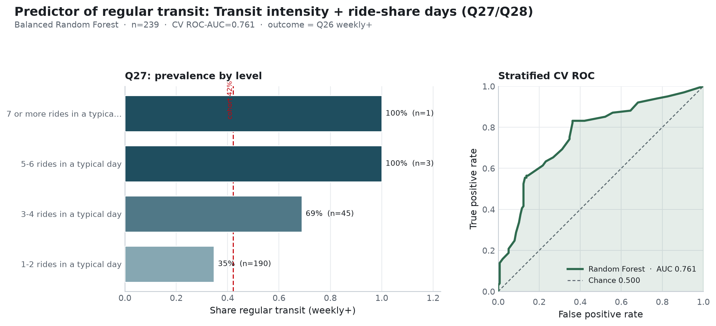
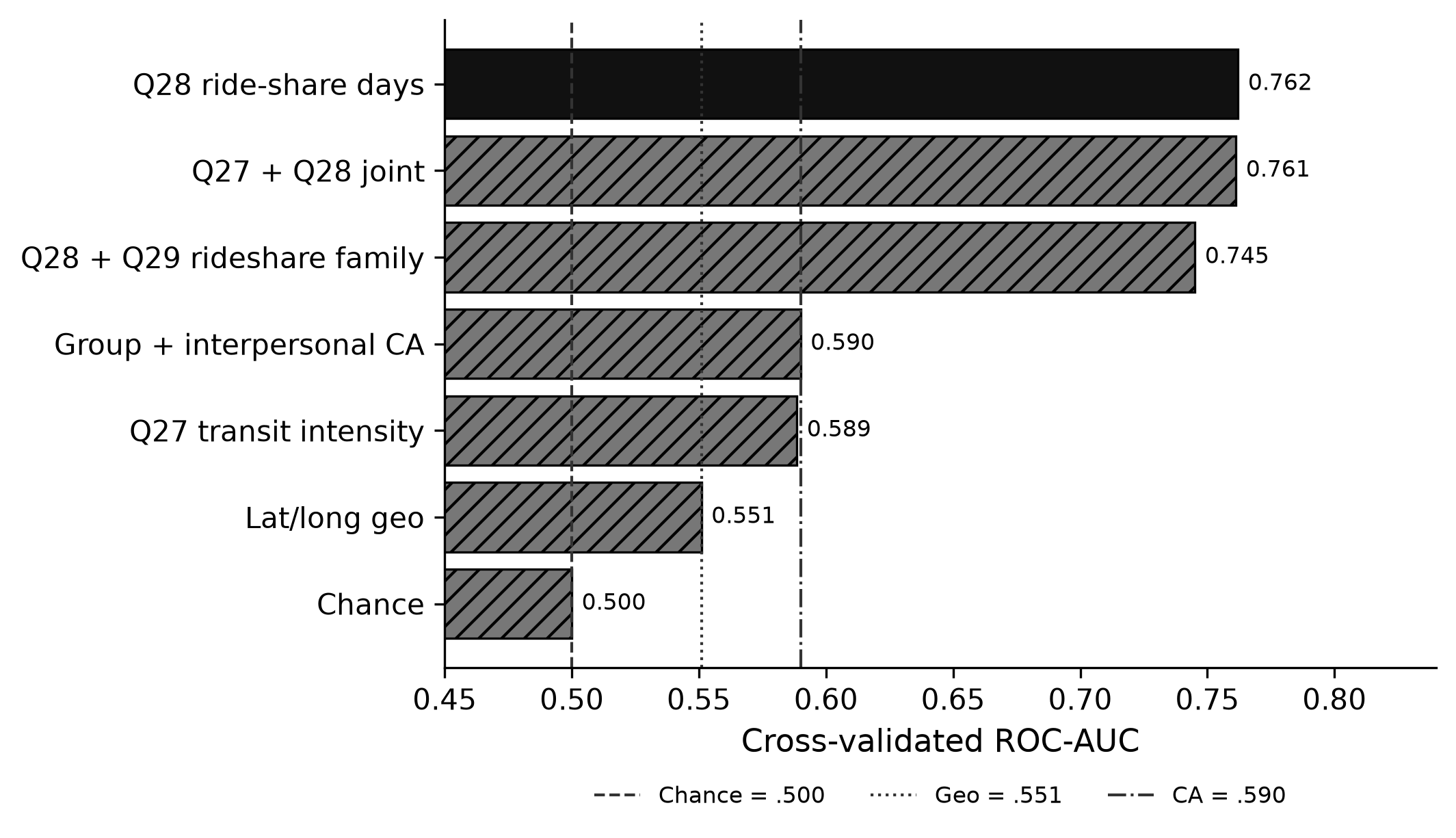
Short answer: Q28 recovers CV ROC-AUC = 0.762 (AP = 0.689; balanced accuracy = 0.730). Q27 recovers AUC = 0.589—matching the CA benchmark (0.590 (McCroskey, 1970))—and the joint Q27+Q28 forest reaches AUC = 0.761 (Δ = −0.001 vs Q28 alone). Ride-share days, not transit-day intensity, carry the usable discrimination.
Figure Figure 1 plots Q27 and Q28 prevalence and ROC curves, and Figure Figure 2 contrasts their head-to-head AUCs against the geo/CA benchmarks.
Q27 prevalence / ROC and Q28 prevalence / ROC
Q27, Q28, joint model vs geo/CA/chance
1.1 Descriptive gradients
Q27 (n = 239). Respondents reporting more rides on a typical transit day are more often weekly+ riders, but most of the sample sits in the lowest intensity bin (Table Table 2):
Q27 intensity distribution by regular transit status.
Q27 |
n | % regular |
|---|---|---|
| 1–2 rides / typical day | 190 | 34.7% |
| 3–4 rides / typical day | 45 | 68.9% |
| 5–6 rides / typical day | 3 | 100% |
| 7+ rides / typical day | 1 | 100% |
Q28 (n = 241). Regular-transit prevalence rises steeply with ride-share days (Table Table 3):
Q28 ride-share days by regular transit status.
Q28 |
n | % regular |
|---|---|---|
| Never | 70 | 15.7% |
| 0–1 days a month | 47 | 23.4% |
| 2–4 days a month | 65 | 52.3% |
| 4–8 days a month | 42 | 69.0% |
| 8 or more days a month | 17 | 94.1% |
1.2 Random Forest performance (stratified CV)
Table Table 4 reports the stratified-CV performance for the Q27/Q28 forests.
Q27 and Q28 predicting regular transit.
| Model | n | ROC-AUC | Avg. precision | Balanced acc. | F1 |
|---|---|---|---|---|---|
Q28 only |
241 | 0.762 | 0.689 | 0.730 | 0.702 |
Q27 + Q28 |
239 | 0.761 | 0.690 | 0.696 | 0.667 |
Q28 + Q29 (rideshare family) |
233 | 0.745 | 0.655 | 0.731 | 0.709 |
Q27 only |
239 | 0.589 | 0.513 | 0.623 | 0.467 |
| CA RF benchmark | 241 | 0.590 | — | — | — |
| Geo RF benchmark | 241 | 0.551 | — | — | — |
| Chance | — | 0.500 | — | 0.500 | — |
Permutation importance in the joint Q27 + Q28 forest ranks Q28 (mean \(\Delta\)AUC = 0.240) far above Q27 (0.041). Adding Q29 (rides on a typical ride-share day) to Q28 does not improve AUC over Q28 alone (rideshare family AUC = 0.745).
1.3 Interpretation
- Significance for traditional ML. Among mobility self-reports tested as reverse predictors of weekly+ transit,
Q28is the dominant signal—exceeding survey geolocation by +0.211 AUC (0.762 vs 0.551) and group/interpersonal CA by +0.172 (0.762 vs 0.590). A single categorical ride-share-days item recovers AP = 0.689 and balanced accuracy = 0.730. Q27’s limited role. Intensity-on-use-days is associated with regular ridership but is sparse above 1–2 rides (n = 3 and n = 1 in the top bins) and yields AUC = 0.589. It is also conceptually adjacent to theQ26outcome (both describe public-transit behavior), so that AUC should not be over-interpreted as an independent lifestyle cue.- Joint model.
Q27does not meaningfully liftQ28; the joint forest is essentially a ride-share-days classifier. For persona-tier design, this reinforces treating ride-share exposure as the high-value transit cue in tabular learners (docs/factor_feature_importance.mdlikewise ranksQ28first when predicting CA). - Non-causal caveat. Same-wave self-reports cannot separate multimodality, urbanicity, income, or common method variance between
Q26andQ28.
Sources: ca-personas covariate-transit-rf --specs q27_intensity q28_days q27_q28 · src/ca_personas/transit_covariate_rf.py · artifacts outputs/transit_covariate_rf/{q27_intensity,q28_days,q27_q28}/ · github.com/Exios66/psych755-jjb
2 What questions or uncertainties remain?
Would Q28 retain its lift after conditioning on city density or car access? Does Q27 help within the regular-rider subgroup for intensity forecasting even though it weakly predicts the weekly+ threshold?
Answered in follow-ups: Q28’s lift after car conditioning is addressed by q28_conditioned_on_car.qmd (AUC 0.665 → 0.730 with Q21); the within-rider intensity question by q27_intensity_among_riders.qmd (best AUC ≈ 0.549 — no usable signal). CA-plus-mobility joint models and multiply-imputed head-to-heads complete the picture in ca_mobility_joint_predicts_transit.qmd and mi_head_to_head.qmd.
Formal write-up: docs/secondary_rq_q27_q28_predict_transit.md