Classical ML baselines for CA prediction
Full stage-one model suite on persona information tiers
Notebook: notebooks/stage_one_ml_baseline.ipynb
Code: src/ca_personas/ml_baseline.py
CLI: ca-personas ml-baseline
Artifacts: outputs/ml_baseline/
Companion comparison: ml_vs_llm.md
1 Research role
Before asking whether an LLM stereotypes CA from persona prompts, we need a tabular ceiling / floor: how well do standard and modern regressors recover the same PRCA targets from the same cumulative feature sets?
| Tier | Features (available in full File A/B/C) |
|---|---|
demos |
Age, Sex, Country of residence, Student status (base demographics layer; optional ethnicity/nationality/language when present) |
employment |
+ Employment status |
geo |
+ survey lat/long |
transit |
+ Q26–Q29, Q20, Q21 |
Targets. gt_group_ca, gt_interpersonal_ca (PRCA subscales, 6–30).
Model suite (7 learners). The stage-one baseline is no longer RF + k-NN alone. We evaluate a deliberately mixed suite so the LLM comparison is not tied to one inductive bias:
| Family | Model | Role |
|---|---|---|
| Linear | Ridge, Elastic Net | Strong regularized linear baselines after one-hot + scaling |
| Instance | k-NN (k = 3, distance-weighted) | Local nonparametric reference |
| Tree ensemble | Random Forest (200 trees) | Classic nonlinear tabular baseline from earlier memos |
| Boosting | Hist. Gradient Boosting, XGBoost | Modern tree boosters |
| Neural | MLP (1×32 hidden, Adam) | Small feed-forward neural net on the same features |
Evaluation. Shuffled 5-fold CV (random_state=42) on the full analytic cohort (N = 241); predictions clipped to [6, 30]; primary metric = MAE (aligned with LLM absolute error), plus RMSE, R², and qualitative band accuracy.
2 Full-cohort results (N = 241)
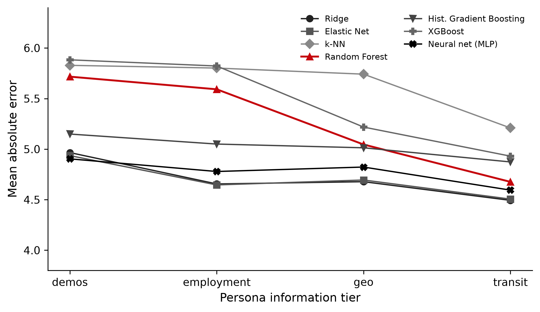
Figure. Group-CA mean absolute error by persona tier for all seven models (seed = 42).
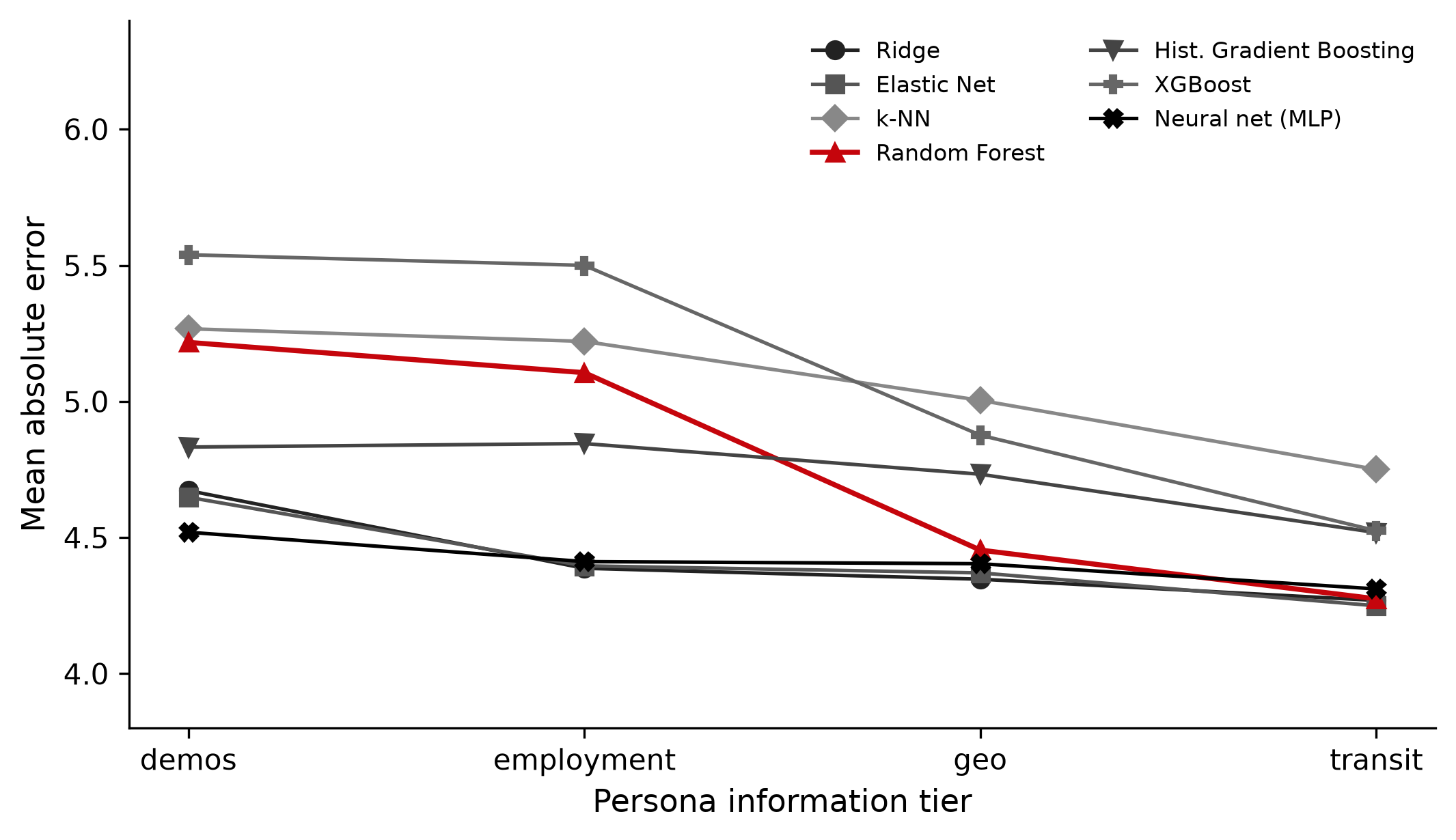
Figure. Interpersonal-CA MAE by persona tier for the same suite.
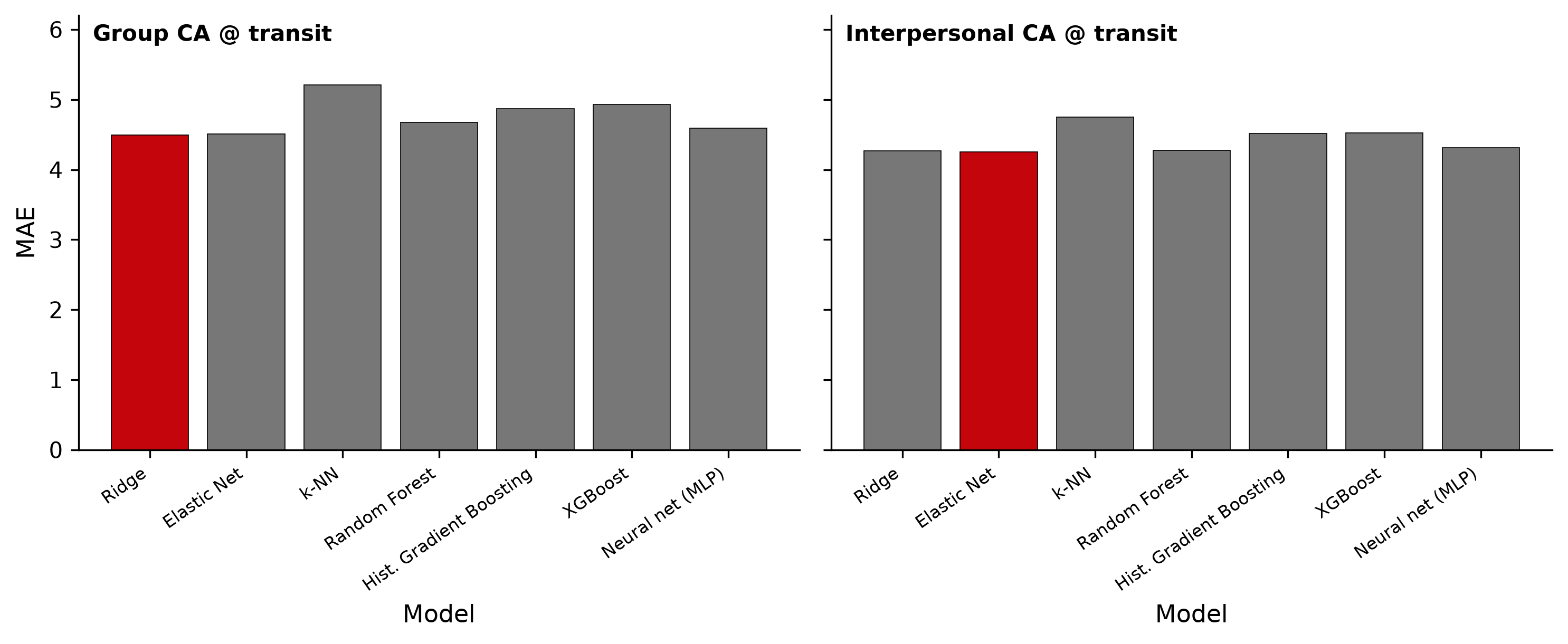
Figure. Transit-tier MAE by model (best model highlighted).
2.1 Group CA — MAE by model × tier (↓ better)
| Model | demos | employment | geo | transit |
|---|---|---|---|---|
| Ridge | 4.97 | 4.66 | 4.68 | 4.49 |
| Elastic Net | 4.94 | 4.65 | 4.69 | 4.51 |
| k-NN | 5.83 | 5.84 | 5.74 | 5.21 |
| Random Forest | 5.72 | 5.59 | 5.05 | 4.68 |
| Hist. Gradient Boosting | 5.15 | 5.05 | 5.01 | 4.87 |
| XGBoost | 5.81 | 5.90 | 5.26 | 4.99 |
| Neural net (MLP) | 4.90 | 4.78 | 4.82 | 4.59 |
2.2 Interpersonal CA — MAE by model × tier
| Model | demos | employment | geo | transit |
|---|---|---|---|---|
| Ridge | 4.67 | 4.39 | 4.35 | 4.27 |
| Elastic Net | 4.65 | 4.40 | 4.37 | 4.25 |
| k-NN | 5.26 | 5.25 | 5.00 | 4.75 |
| Random Forest | 5.22 | 5.11 | 4.45 | 4.27 |
| Hist. Gradient Boosting | 4.83 | 4.85 | 4.73 | 4.52 |
| XGBoost | 5.57 | 5.47 | 4.93 | 4.51 |
| Neural net (MLP) | 4.52 | 4.41 | 4.40 | 4.31 |
2.3 Best model per tier × target (leaderboard)
| Tier | Target | Best model | Best MAE | Band acc. | Gap to 2nd |
|---|---|---|---|---|---|
| demos | group | MLP | 4.90 | 0.274 | 0.032 |
| demos | interpersonal | MLP | 4.52 | 0.369 | 0.128 |
| employment | group | Elastic Net | 4.65 | 0.456 | 0.010 |
| employment | interpersonal | Ridge | 4.39 | 0.456 | 0.009 |
| geo | group | Ridge | 4.68 | 0.452 | 0.017 |
| geo | interpersonal | Ridge | 4.35 | 0.440 | 0.023 |
| transit | group | Ridge | 4.49 | 0.481 | 0.012 |
| transit | interpersonal | Elastic Net | 4.25 | 0.448 | 0.020 |
Seeded tables: outputs/ml_baseline/ml_baseline_mae_pivot_*.csv, ml_baseline_leaderboard.csv (seed = 42).
3 Interpretation
Linear models are the strongest floor at rich tiers. On this cohort, Ridge / Elastic Net beat Random Forest for group CA at every tier except the mid-tier RF spike at
geo(RF 5.05 vs Ridge 4.68). Attransit, Ridge reaches group MAE 4.49 — 0.18 better than RF (4.68). Demographics + mobility self-reports look closer to a weak linear mapping than a deep tree interaction for these PRCA subscales.The small MLP wins only the sparse
demostier. MLP is best atdemosfor both targets (group 4.90; interpersonal 4.52), but loses transit interpersonal to Elastic Net (4.25 vs MLP 4.31) and employment interpersonal to Ridge (4.39 vs MLP 4.41). Treat MLP as a useful nonlinear check, not a new ceiling.Boosters do not dominate. HistGradientBoosting and XGBoost sit between RF and the linear/MLP pack on most tiers. With N = 241, mixed categoricals, and only a handful of features even at
transit(13 columns before one-hot), aggressive boosting overfits relative to Ridge. This is an important negative result for “always use XGBoost on tabular data.”k-NN remains the weak baseline. Distance-weighted k-NN is worst or near-worst at every tier (group transit MAE 5.21), confirming that local demographic neighbors are a poor CA proxy.
Adding context still helps the better models. Ridge group MAE falls from 4.97 (
demos) → 4.49 (transit) (−0.48). RF still shows the familiar path 5.72 → 4.68. The largest stepwise gains for RF remainemployment→geoandgeo→transit; linear models gain most from employment, then transit.Band accuracy stays modest. Even the best transit group model (Ridge) reaches band accuracy 0.481 — better than chance among three bands, but far from reliable low/moderate/high recovery from demographics + context alone. R² peaks around 0.13–0.15 at transit for the best models.
Implication for LLM personification. The relevant classical floor is no longer “RF = 4.68.” Use the suite best at each tier (4.25–4.49 at transit). An LLM that only matches RF but loses to Ridge/Elastic Net is still behind the tabular ceiling. Live full-cohort vLLM group MAEs (best pooled: DeepSeek-R1-Distill-Llama-8B under v2 packaging 5.02; prompt-v1 range 5.22–6.02) remain above the suite floor here (
index.qmd).
4 Link to the LLM manuscript
- These MAE numbers are the classical reference for
ml_vs_llm.md: an LLM tier “helps” only if it approaches or beats the best suite MAE on the same tier (not RF alone). - Because even the best suite MAE remains 4.25–4.49 points at
transit, persona prompts that land in that range are competitive with tabular learners — not magical. - Feature-importance diagnostics (factor_feature_importance.md; memo) still use RF/TreeSHAP to show which covariates carry signal (Q28 ranks first for predicting CA); the expanded suite answers how high that signal goes across model classes.
5 Reproducibility
# Requires sibling File A/B/C (../sibling_data or CA_SIBLING_DATA=/tmp/sibling_data)
pip install -e .
ca-personas ml-baseline --join inner --seed 42 --output-dir outputs/ml_baseline

# Or execute the notebook
jupyter nbconvert --to notebook --execute notebooks/stage_one_ml_baseline.ipynb
Optional model subset:
ca-personas ml-baseline --models ridge elastic_net random_forest xgboost mlpSeeded metrics live in outputs/ml_baseline/ml_baseline_metrics.csv (plus leaderboard and MAE pivots).